This introductory workshop was given by Ramiro Aznar on May 26, 2016 at . As taught, it was 1h 30' hours long.

Speaker: Ramiro Aznar · ramiroaznar@cartodb.com · @ramiroaznar
May 26th 2016
Máster en Gestión de Desastres· UCM y UPM · Madrid
Slides

http://bit.ly/intro-mgd

Importing datasets
Getting your data ready
Making a map
Mini-Project: Subterranean evacuation routes

Introduction to CartoDB Workshop for MSc Disasters Management students

1. Importing datasets

1. 1. Supported Geospatial Data Files

CartoDB supports the following geospatial data formats to upload vector data*:

Shapefile.
KML.
KMZ.
GeoJSON**.
CSV.
Spreedsheets.
GPX.
OSM.

1. 2. Common importing errors

Dataset too large:
- File size limit: 150 Mb (free).
- Import row limit: 500,000 rows (free).
- Solution: split your dataset into smaller ones, import them into CartoDB and merge them.
Malformed CSV:
- Solution: check termination lines, header…
Encoding:
- Solution: Save with Encoding > UTF-8 with BOM in Sublime Text.
Shapefile missing files:
- Missing any of the following files within the compressed file will produce an importing error:
  - .shp: contains the geometry. REQUIRED.
  - .shx: contains the shape index. REQUIRED.
  - .prj: contains the projection. REQUIRED.
  - .dbf: contains the attributes. REQUIRED.
- Other auxiliary files such as .sbn, .sbx or .shp.xml are not REQUIRED.
- Solution: make sure to add all required files.
Duplicated id fields:
- Solution: check your dataset, remove or rename fields containing the id keyword.
Format not supported:
- URLs -that are not points to a file- are not supported by CartoDB.
- Solution: check for missing url parameters or download the file into your local machine, import it into CartoDB.

Other importing errors and their codes can be found here.

Practice! Download and import into CartoDB the following datasets:

hospitales, download dataset as csv file.
estaciones, download dataset as shapefile file.
lineas, download dataset as shapefile file.
escenarios, download dataset as shapefile file.

*Check this link in order to view the OpenStreetMap bounding box where some of the data was extracted (as a .osm file).

2. Getting your data ready

2. 1. Geocoding

If you have a column with longitude coordinates and another with latitude coordinates, CartoDB will automatically detect and covert values into the_geom. If this is not the case, CartoDB can help you by turning the named places into best guess of latitude-longitude coordinates:

By Lon/Lat Columns.
By City Names.
By Admin. Regions.
By Postal Codes.
By IP Addresses.
By Street Addresses.

Know more about geocoding in CartoDB in this tutorial.

Practice! Georeference the hospitales dataset.

2. 2. Datasets

Search, connect and disable syncronization of the following datasets:

Populated Places [ne_10m_populated_places_simple]: City and town points.
World Borders [world_borders]: World countries borders.
European countries [ne_adm0_europe]: European countries geometries.

2. 3. Selecting

Selecting all the columns:

SELECT
  *
FROM
  ne_10m_populated_places_simple;

Selecting some columns:

SELECT
  cartodb_id,
  name as city,
  adm1name as region,
  adm0name as country,
  pop_max,
  pop_min
FROM 
  ne_10m_populated_places_simple

Selecting distinc values:

SELECT DISTINCT
  adm0name as country
FROM 
  ne_10m_populated_places_simple

Selecting aggregated values:

SELECT
  count(*) as total_rows --other aggregated functions: sum(), avg()...
FROM 
  ne_10m_populated_places_simple

2. 4. Filtering

filtering

Filtering numeric fields:

SELECT 
  * 
FROM 
  ne_10m_populated_places_simple
WHERE
  pop_max > 5000000;

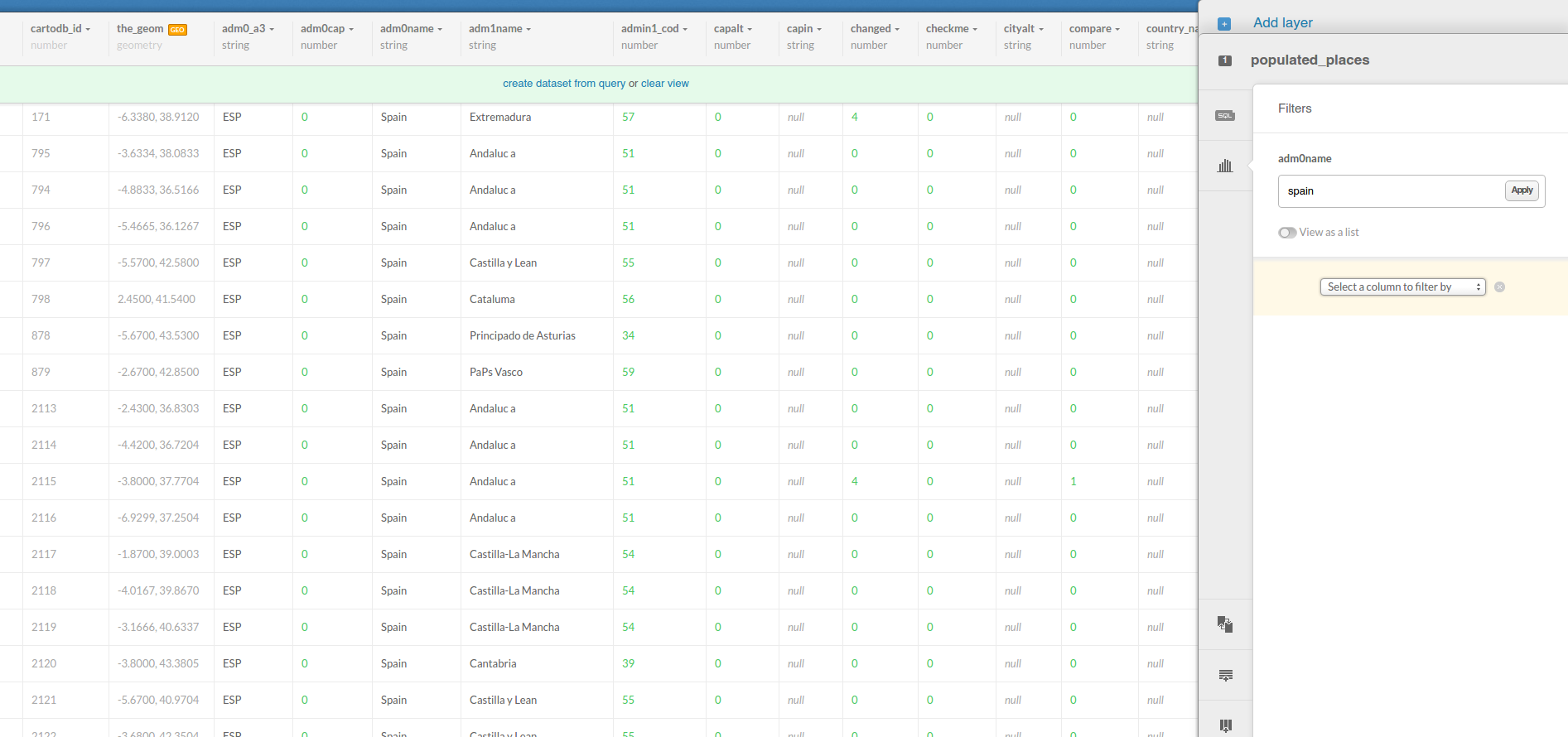
Filtering character fields:

SELECT 
  *
FROM 
  ne_10m_populated_places_simple
WHERE 
  adm0name ilike 'spain'

Filtering a range:

SELECT 
  *
FROM 
  ne_10m_populated_places_simple
WHERE 
  name in ('Madrid', 'Barcelona')
AND
  adm0name ilike 'spain'

2. 5. Ordering and limiting results:

Ordering results:

SELECT 
  cartodb_id,
  name as city,
  adm1name as region,
  adm0name as country,
  pop_max
FROM 
  ne_10m_populated_places_simple
WHERE 
  adm0name ilike 'spain'
ORDER BY
  pop_max DESC

Limiting results:

SELECT 
  cartodb_id,
  the_geom_webmercator,
  name as city,
  adm1name as region,
  adm0name as country,
  pop_max
FROM 
  ne_10m_populated_places_simple
WHERE 
  adm0name ilike 'spain'
ORDER BY
  pop_max DESC LIMIT 10

2. 6. Spatial Analysis:

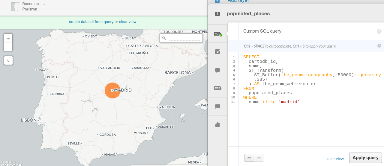
Create a buffer from points:

SELECT
  cartodb_id,
  name,
  ST_Transform(
    ST_Buffer(the_geom::geography, 50000)::geometry
    ,3857
  ) AS the_geom_webmercator
FROM
  ne_10m_populated_places_simple
WHERE
  name ilike 'madrid'

buffer

Know if two geometries intersect:

SELECT
  a.*
FROM
  ne_10m_populated_places_simple a,
  ne_adm0_europe b
WHERE
  ST_Intersects(
    b.the_geom_webmercator,
    a.the_geom_webmercator
  )

intersects

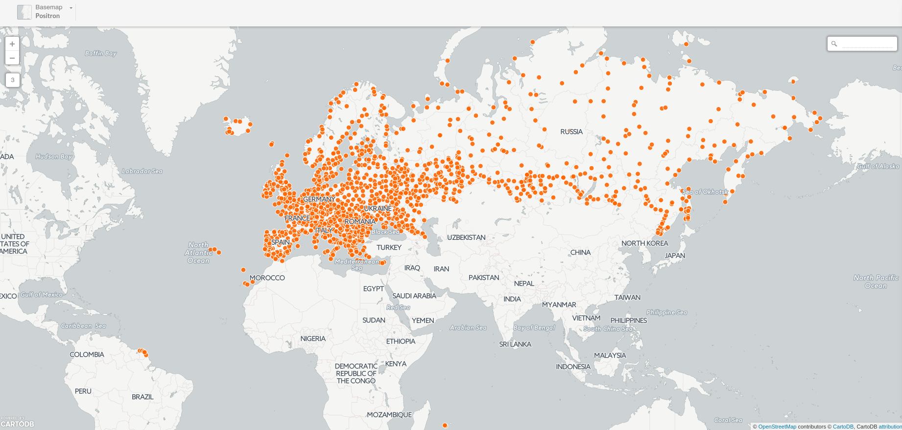
*About ST_Intersects.

Know wether a geometry is within the given range from another geometry:

SELECT
  a.*
FROM
  ne_10m_populated_places_simple a,
  ne_10m_populated_places_simple b
WHERE
    a.cartodb_id != b.cartodb_id
  AND ST_DWithin(
      a.the_geom_webmercator,
      b.the_geom_webmercator,
      150000
    )
  AND a.adm0name = 'Spain'
  AND b.adm0name = 'Spain'

dwithin

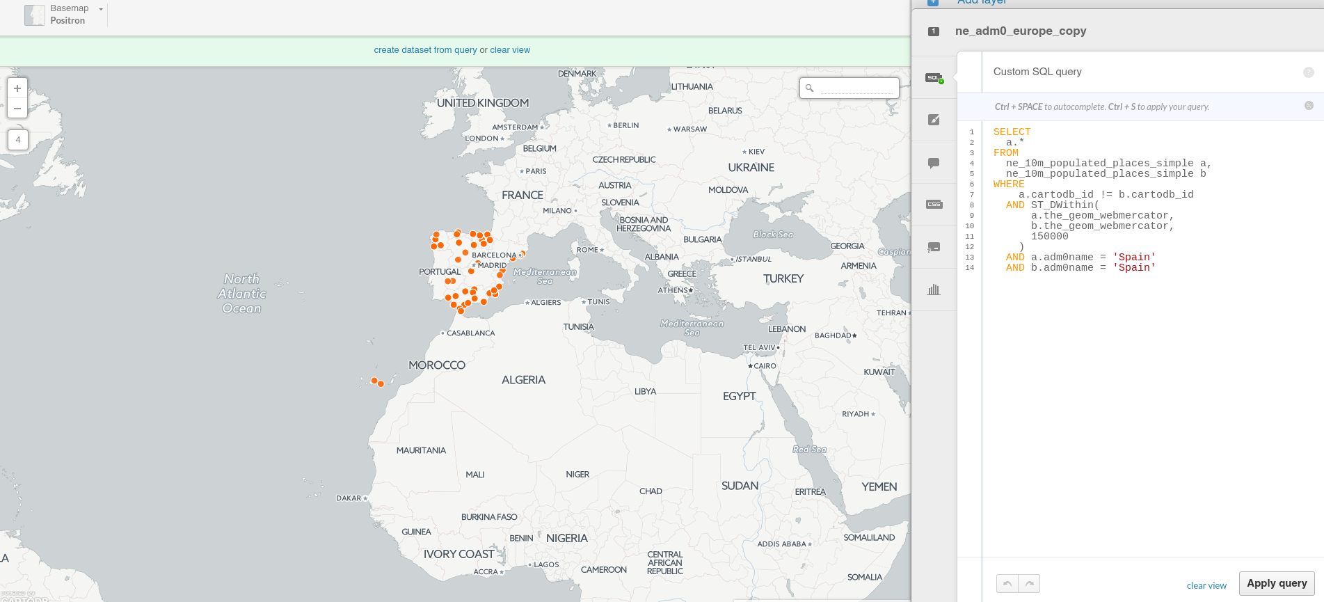
*About ST_DWithin.

Practice! Select metro stations from L1 using the following three methods:

Filtering by (string) range (query).
Selecting stations which intersect with a 100m buffer of the L1 metro line (query).
Selecting stations within a minimun distance of 100m from the L1 metro line (query).

3. Making a map

3. 1. Wizard

Analyzing your dataset… In some cases, when you connect a dataset and click on the MAP VIEW for the first time, the Analyzing dataset dialog appears. This analytical tool analyzes the data in each column, predicts how to visualize this data, and offers you snapshots of the visualized maps. You can select one of the possible map styles, or ignore the analyzing dataset suggestions.

Simple Map.
Cluster Map.
Category Map.
Bubble Map.
Torque Map.
Heatmap Map.
Torque Cat Map.
Intensity Map.
Density Map.
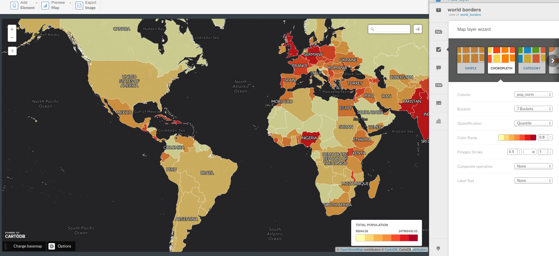
Choropleth Map:

Before making a choropleth map, we need to normalize our target column. So we are going to create two new columns with numeric as data type: new_area and pop_norm. Finally, run the following SQL queries to update their values:

UPDATE
  world_borders
SET
  new_area = round(st_area(the_geom)::numeric, 6)

UPDATE
  world_borders
SET
  pop_norm = pop2005 / new_area

choropleth

Know more about chosing the right map to make here.

3. 2. Styles

Simple Map:

/** simple visualization */

#world_borders{
  polygon-fill: #FF6600;
  polygon-opacity: 0.7;
  line-color: #FFF;
  line-width: 0.5;
  line-opacity: 1;
}

Choropleth Map:

/** choropleth visualization */

#world_borders{
  polygon-fill: #FFFFB2;
  polygon-opacity: 0.8;
  line-color: #FFF;
  line-width: 0.5;
  line-opacity: 1;
}
#world_borders [ pop_norm <= 247992435.530086] {
   polygon-fill: #B10026;
}
#world_borders [ pop_norm <= 4086677.23673585] {
   polygon-fill: #E31A1C;
}
#world_borders [ pop_norm <= 1538732.3943662] {
   polygon-fill: #FC4E2A;
}
#world_borders [ pop_norm <= 923491.374542489] {
   polygon-fill: #FD8D3C;
}
#world_borders [ pop_norm <= 616975.331234902] {
   polygon-fill: #FEB24C;
}
#world_borders [ pop_norm <= 326396.192958792] {
   polygon-fill: #FED976;
}
#world_borders [ pop_norm <= 95044.5589361554] {
   polygon-fill: #FFFFB2;
}

Category Map.
Bubble Map.
Torque Map.
Heatmap Map.
Torque Cat Map.
Intensity Map.
Density Map.

Know more about CartoCSS with our documentation.

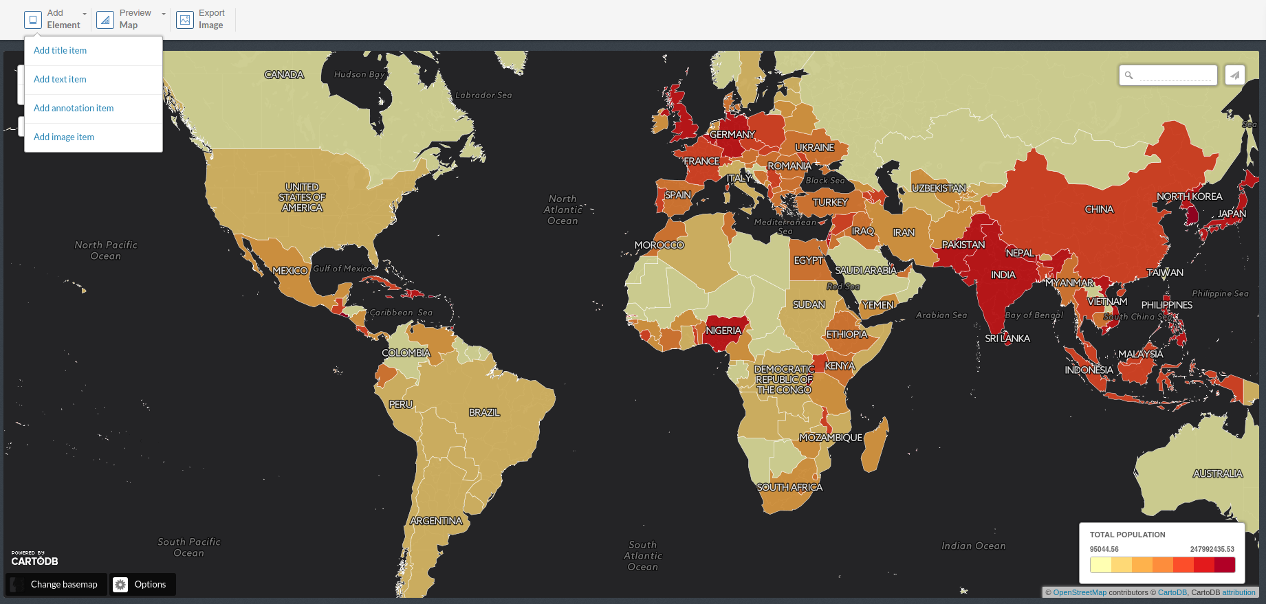
3. 3. Other elements

Basemaps:

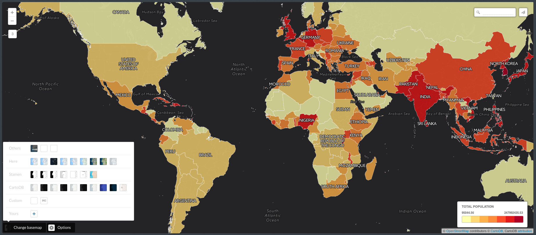
basemap

Options:

options

Legend:

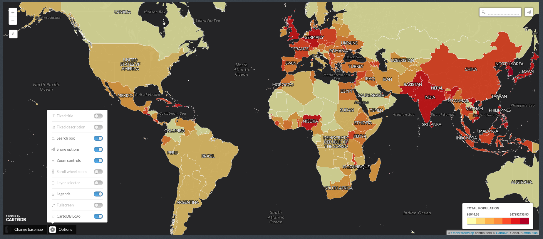
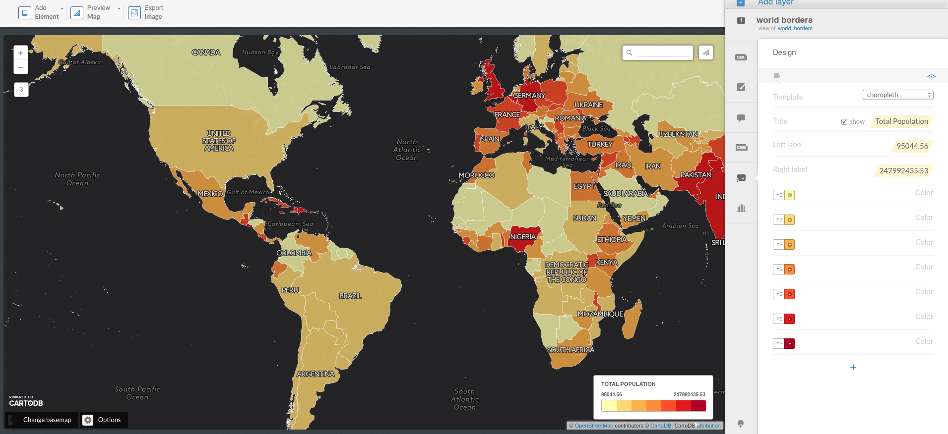
legend

Labels:

intensity

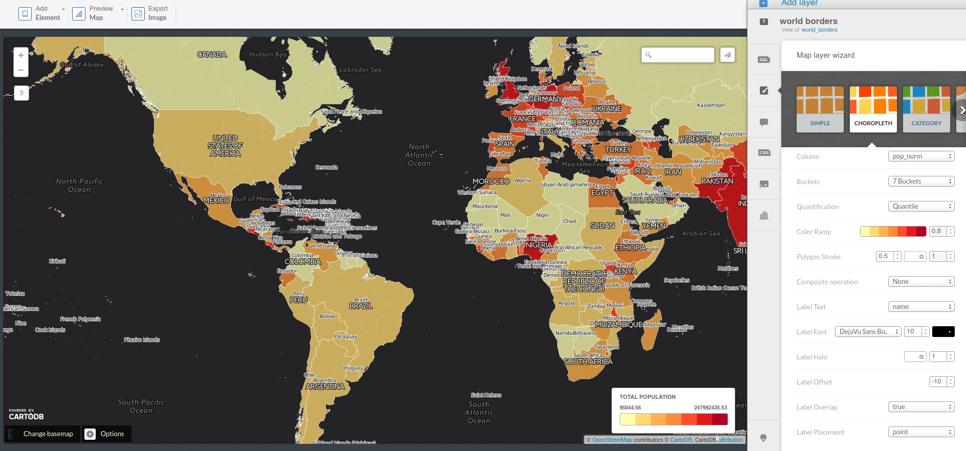
#world_borders::labels {
  text-name: [name];
  text-face-name: 'DejaVu Sans Book';
  text-size: 10;
  text-label-position-tolerance: 10;
  text-fill: #000;
  text-halo-fill: #FFF;
  text-halo-radius: 1;
  text-dy: -10;
  text-allow-overlap: true;
  text-placement: point;
  text-placement-type: simple;
}

Infowindows and tooltip:

infowindows

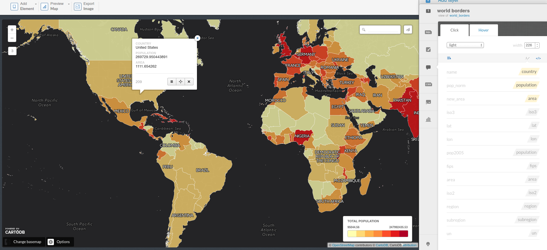
Title, text and images:

elements

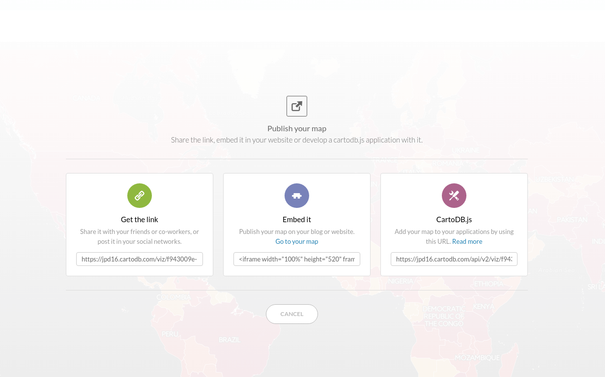
Get the link: https://team.cartodb.com/u/ramirocartodb/viz/0ba65c92-120b-11e6-9ab2-0e5db1731f59/public_map
Embed it:

CartoDB.js [vizJSON file*]: https://team.cartodb.com/u/ramirocartodb/api/v2/viz/0ba65c92-120b-11e6-9ab2-0e5db1731f59/viz.json

Practice! Make the Madrid Metro map as a category map coloring metro lines according to their real colors (CartoCSS).

4. Mini-Project: Subterranean evacuation routes

Practice! Try to answer the following questions using CartoDB:

What are the closest (500m) Metro stations to the three scenarios?
What are the closest (250m) Metro stations to the hospitals?
What are the Mtro lines which connect these set of stations?
What is the best combination (closest Metro station to the scenario - closest Metro station to the hospital)?

Practice! Make a map to visualize your answers (remember that you can create new datasets from your queries). And share it with the rest of your class and social media!

CartoDB Workshops Materials for Teaching Maps