Intermediate CartoDB Workshop for MSc Geo Engineers
- Speaker: Ramiro Aznar · ramiroaznar@cartodb.com · @ramiroaznar
- May 10th 2016
- MSc in Geomatics and Cartographic Engineering · Universidad Politécnica de Madrid · Madrid
- Slides.
http://bit.ly/cdb-upm
Contents
- Importing datasets
- Getting your data ready
- Making a map
- Going spatial with PostGIS
- Webmapping apps with CartoDB.js
Intermediate CartoDB Workshop for MSc Geo Engineers
1. Importing datasets
1. 1. Supported Geospatial Data Files
CartoDB supports the following geospatial data formats to upload vector data*:
Shapefile.KML.KMZ.GeoJSON**.CSV.Spreedsheets.GPX.OSM.
*Importing different geometry types in the same layer or in a FeatureCollection element (GeoJSON) is not supported. More detailed information here. **More detailed information about GeoJSON format here.
1. 2. Common importing errors
- Dataset too large:
- File size limit: 150 Mb (free).
- Import row limit: 500,000 rows (free).
- Solution: split your dataset into smaller ones, import them into CartoDB and merge them.
- Malformed CSV:
- Solution: check termination lines, header…
- Solution: check termination lines, header…
- Encoding:
- Solution:
Save with Encoding>UTF-8 with BOMin Sublime Text.
- Solution:
- Shapefile missing files:
- Missing any of the following files within the compressed file will produce an importing error:
.shp: contains the geometry. REQUIRED..shx: contains the shape index. REQUIRED..prj: contains the projection. REQUIRED..dbf: contains the attributes. REQUIRED.
- Other auxiliary files such as
.sbn,.sbxor.shp.xmlare not REQUIRED. - Solution: make sure to add all required files.
- Missing any of the following files within the compressed file will produce an importing error:
- Duplicated id fields:
- Solution: check your dataset, remove or rename fields containing the
idkeyword.
- Solution: check your dataset, remove or rename fields containing the
- Format not supported:
- URLs -that are not points to a file- are not supported by CartoDB.
- Solution: check for missing url parameters or download the file into your local machine, import it into CartoDB.
- MAYUS extensions not supported:
example.CSVis not supported by CartoDB.- Solution: rename the file.
Other importing errors and their codes can be found here.
2. Getting your data ready
2. 1. Geocoding
If you have a column with longitude coordinates and another with latitude coordinates, CartoDB will automatically detect and covert values into the_geom. If this is not the case, CartoDB can help you by turning the named places into best guess of latitude-longitude coordinates:
- By Lon/Lat Columns.
- By City Names.
- By Admin. Regions.
- By Postal Codes.
- By IP Addresses.
- By Street Addresses.
Know more about geocoding in CartoDB:
- In this tutorial.
- In our Location Data Services website.
- In our documentation.
2. 2. Datasets
- Populated Places [
ne_10m_populated_places_simple]: City and town points. - World Borders [
world_borders]: World countries borders. - Emerged Lands [
ne_50m_land]: World emerged lands.
2. 3. Selecting
- Selecting all the columns:
SELECT
  *
FROM
  ne_10m_populated_places_simple;
- Selecting some columns:
SELECT
  cartodb_id,
  name as city,
  adm1name as region,
  adm0name as country,
  pop_max,
  pop_min
FROM
  ne_10m_populated_places_simple
- Selecting distinc values:
SELECT DISTINCT
  adm0name as country
FROM
  ne_10m_populated_places_simple
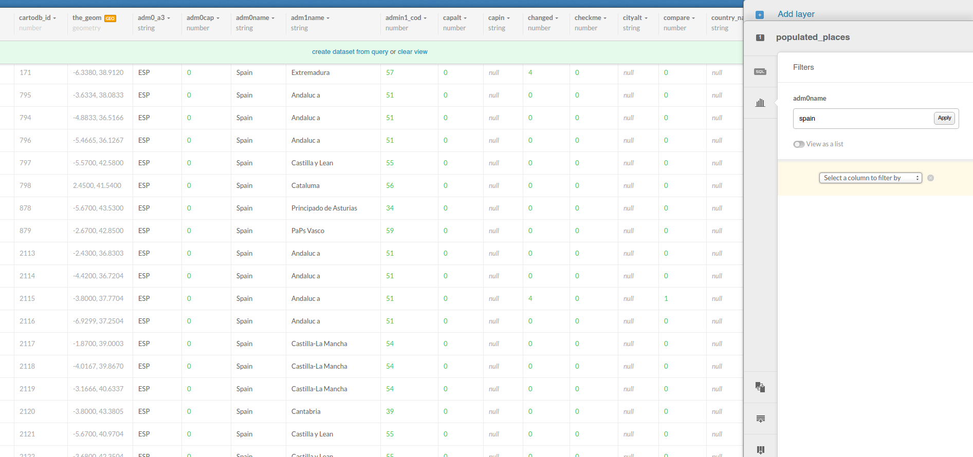
2. 4. Filtering
- Filtering numeric fields:
SELECT
  *
FROM
  ne_10m_populated_places_simple
WHERE
  pop_max > 5000000;
- Filtering character fields:
SELECT
  *
FROM
  ne_10m_populated_places_simple
WHERE
  adm0name ilike 'spain'
- Filtering a range:
SELECT
  *
FROM
  ne_10m_populated_places_simple
WHERE
  name in ('Madrid', 'Barcelona')
AND
  adm0name ilike 'spain'
- Combining character and numeric filters:
SELECT
  *
FROM
  ne_10m_populated_places_simple
WHERE
  name in ('Madrid', 'Barcelona')
AND
  adm0name ilike 'spain'
AND
  pop_max > 5000000
2. 5. Others:
- Selecting aggregated values:
SELECT
  count(*) as total_rows
FROM
  ne_10m_populated_places_simple
SELECT
  sum(pop_max) as total_pop_spain
FROM
  ne_10m_populated_places_simple
WHERE
  adm0name ilike 'spain'
SELECT
  avg(pop_max) as avg_pop_spain
FROM
  ne_10m_populated_places_simple
WHERE
  adm0name ilike 'spain'
- Ordering results:
SELECT
  cartodb_id,
  name as city,
  adm1name as region,
  adm0name as country,
  pop_max
FROM
  ne_10m_populated_places_simple
WHERE
  adm0name ilike 'spain'
ORDER BY
  pop_max DESC
- Limiting results:
SELECT
  cartodb_id,
  name as city,
  adm1name as region,
  adm0name as country,
  pop_max
FROM
  ne_10m_populated_places_simple
WHERE
  adm0name ilike 'spain'
ORDER BY
  pop_max DESC LIMIT 10
3. Making a map
3. 1. Wizard
Analyzing your dataset… In some cases, when you connect a dataset and click on the MAP VIEW for the first time, the Analyzing dataset dialog appears. This analytical tool analyzes the data in each column, predicts how to visualize this data, and offers you snapshots of the visualized maps. You can select one of the possible map styles, or ignore the analyzing dataset suggestions.
- Simple Map.
- Cluster Map.
- Category Map.
- Bubble Map.
- Torque Map.
- Heatmap Map.
- Torque Cat Map.
- Intensity Map.
-
Density Map.
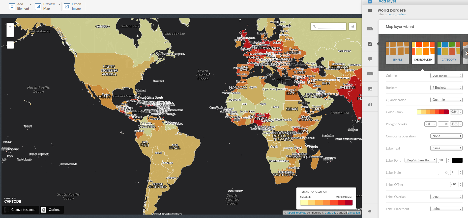
- Choropleth Map:
Before making a choropleth map, we need to normalize our target column. So we are going to create two new columns with numeric as data type: new_area and po_norm. Finally, run the following SQL queries to update their values:
UPDATE
  world_borders
SET
  new_area = round(st_area(the_geom)::numeric, 6)
UPDATE
  world_borders
SET
  pop_norm = pop2005 / new_area
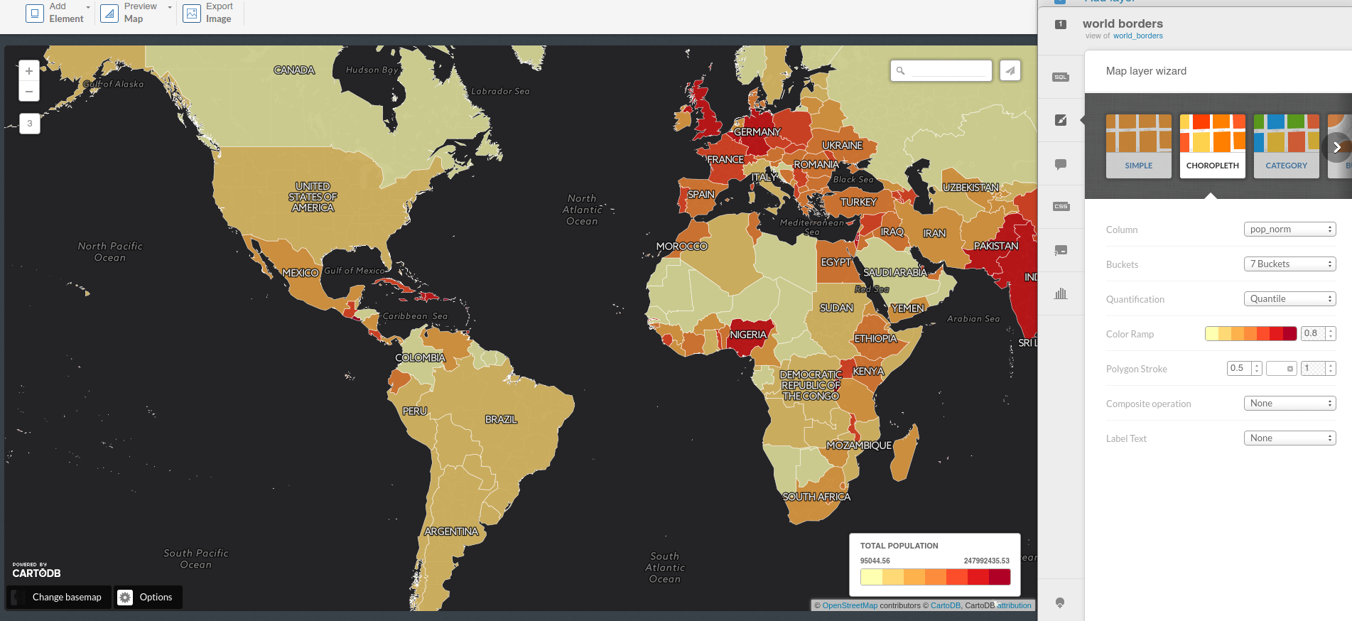
Know more about chosing the right map to make here.
3. 2. Styles
- Simple Map:
/** simple visualization */

#world_borders{
  polygon-fill: #FF6600;
  polygon-opacity: 0.7;
  line-color: #FFF;
  line-width: 0.5;
  line-opacity: 1;
}
- Choropleth Map:
/** choropleth visualization */

#world_borders{
  polygon-fill: #FFFFB2;
  polygon-opacity: 0.8;
  line-color: #FFF;
  line-width: 0.5;
  line-opacity: 1;
}
#world_borders [ pop_norm <= 247992435.530086] {
   polygon-fill: #B10026;
}
#world_borders [ pop_norm <= 4086677.23673585] {
   polygon-fill: #E31A1C;
}
#world_borders [ pop_norm <= 1538732.3943662] {
   polygon-fill: #FC4E2A;
}
#world_borders [ pop_norm <= 923491.374542489] {
   polygon-fill: #FD8D3C;
}
#world_borders [ pop_norm <= 616975.331234902] {
   polygon-fill: #FEB24C;
}
#world_borders [ pop_norm <= 326396.192958792] {
   polygon-fill: #FED976;
}
#world_borders [ pop_norm <= 95044.5589361554] {
   polygon-fill: #FFFFB2;
}
- Category Map.
- Bubble Map.
- Torque Map.
- Heatmap Map.
- Torque Cat Map.
- Intensity Map.
- Density Map.
Know more about CartoCSS with our documentation.
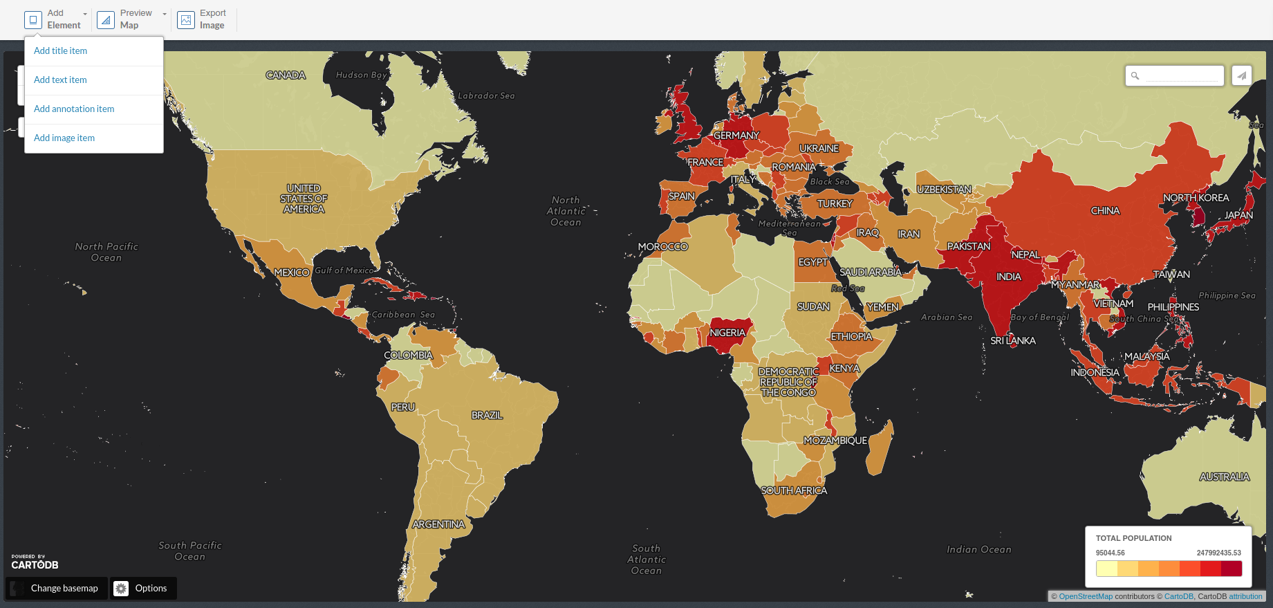
3. 3. Other elements
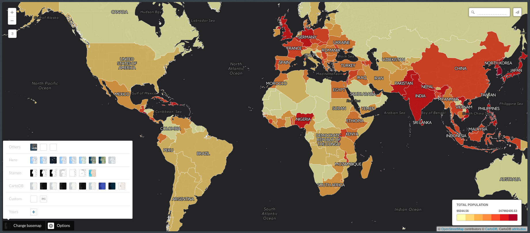
- Basemaps:
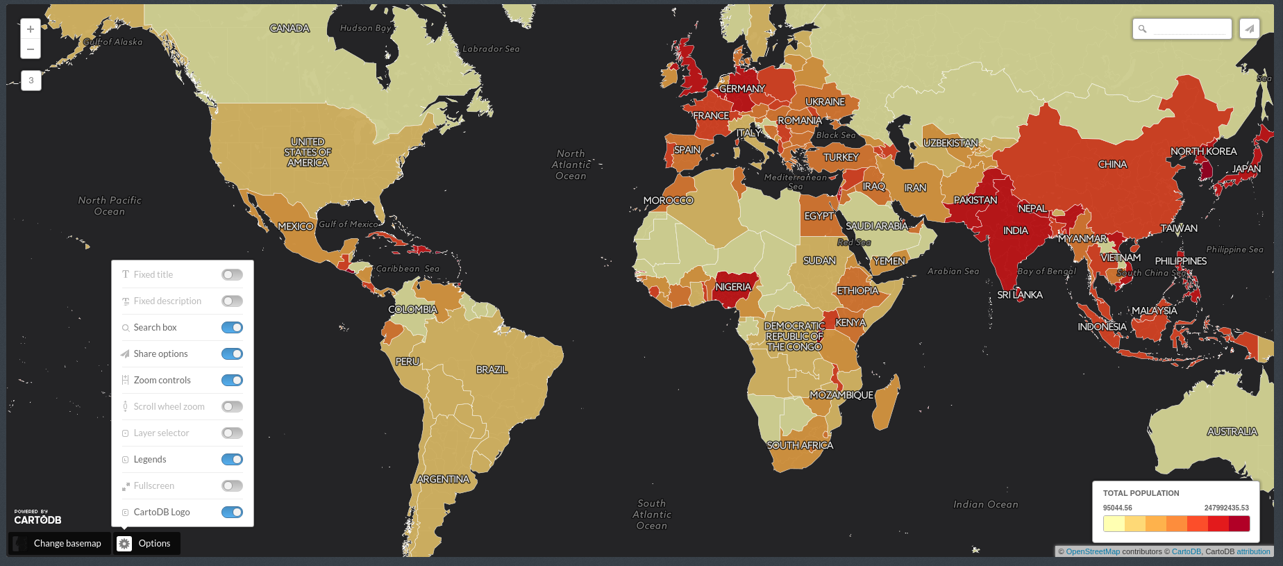
- Options:
- Legend:
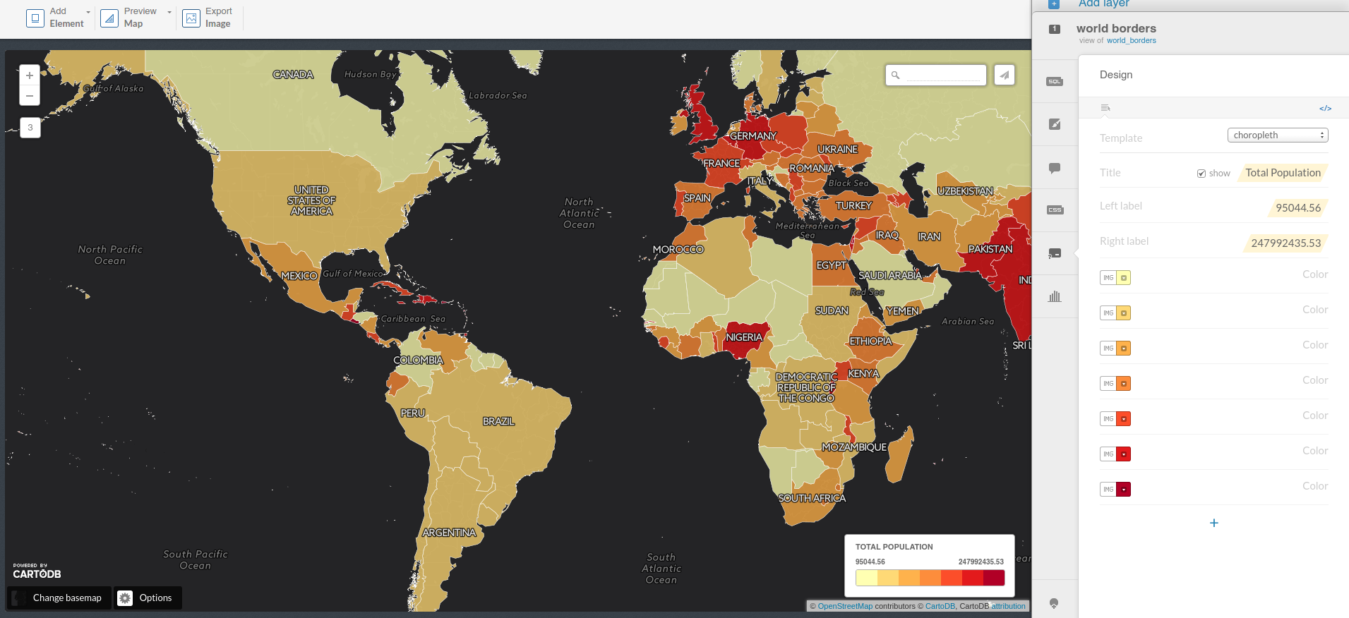
<div class='cartodb-legend choropleth'>
<div class="legend-title">Total Population</div>
<ul>
	<li class="min">
		95044.56
	</li>
	<li class="max">
		247992435.53
	</li>
	<li class="graph count_441">
	<div class="colors">
	<div class="quartile" style="background-color:#FFFFB2"></div>
	<div class="quartile" style="background-color:#FED976"></div>
	<div class="quartile" style="background-color:#FEB24C"></div>
	<div class="quartile" style="background-color:#FD8D3C"></div>
	<div class="quartile" style="background-color:#FC4E2A"></div>
	<div class="quartile" style="background-color:#E31A1C"></div>
	<div class="quartile" style="background-color:#B10026"></div>
	</div>
	</li>
</ul>
</div>
- Labels:
#world_borders::labels {
  text-name: [name];
  text-face-name: 'DejaVu Sans Book';
  text-size: 10;
  text-label-position-tolerance: 10;
  text-fill: #000;
  text-halo-fill: #FFF;
  text-halo-radius: 1;
  text-dy: -10;
  text-allow-overlap: true;
  text-placement: point;
  text-placement-type: simple;
}
- Infowindows and tooltip:
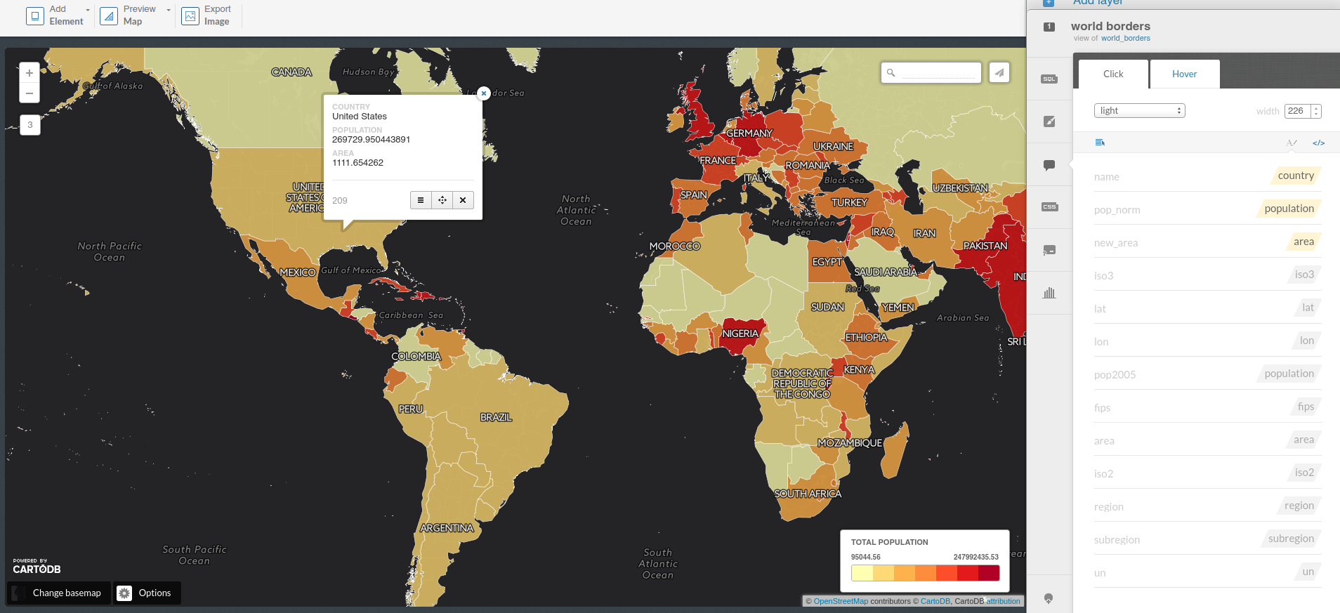
<div class="cartodb-popup v2">
  <a href="#close" class="cartodb-popup-close-button close">x</a>
  <div class="cartodb-popup-content-wrapper">
    <div class="cartodb-popup-content">
      <h4>country</h4>
      <p></p>
      <h4>population</h4>
      <p></p>
      <h4>area</h4>
      <p></p>
    </div>
  </div>
  <div class="cartodb-popup-tip-container"></div>
</div>
- Title, text and images:
3. 4. Share your map!
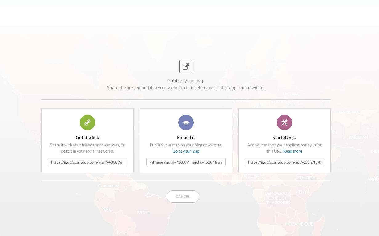
-
Get the link: https://team.cartodb.com/u/ramirocartodb/viz/0ba65c92-120b-11e6-9ab2-0e5db1731f59/public_map
-
Embed it:
- CartoDB.js [vizJSON file*]: https://team.cartodb.com/u/ramirocartodb/api/v2/viz/0ba65c92-120b-11e6-9ab2-0e5db1731f59/viz.json
*BONUS: JSONView, a Google Chrome extension and Pretty JSON, a Sublime Text plugin to visualize json files are good resources.
4. Going spatial with PostGIS
4. 1. Working with projections
4. 1. 1. geometry vs. geography
-
Geometryuses a cartesian plane to measure and store features (CRS units):The basis for the PostGIS
geometrytype is a plane. The shortest path between two points on the plane is a straight line. That means calculations on geometries (areas, distances, lengths, intersections, etc) can be calculated using cartesian mathematics and straight line vectors. -
Geographyuses a sphere to measure and store features (Meters):The basis for the PostGIS
geographytype is a sphere. The shortest path between two points on the sphere is a great circle arc. That means that calculations on geographies (areas, distances, lengths, intersections, etc) must be calculated on the sphere, using more complicated mathematics. For more accurate measurements, the calculations must take the actual spheroidal shape of the world into account, and the mathematics becomes very complicated indeed.
More about the geography type can be found here and here.

4. 1. 2. the_geom and the_geom_webmercator
the_geomEPSG:4326. Unprojected coordinates in decimal degrees (Lon/Lat). WGS84 Spheroid.the_geom_webmercatorEPSG:3857. UTM projected coordinates in meters. This is a conventional Coordinate Reference System, widely accepted as a ‘de facto’ standard in webmapping.
In CartoDB, the_geom_webmercator column is the one we see represented in the map. Know more about projections:
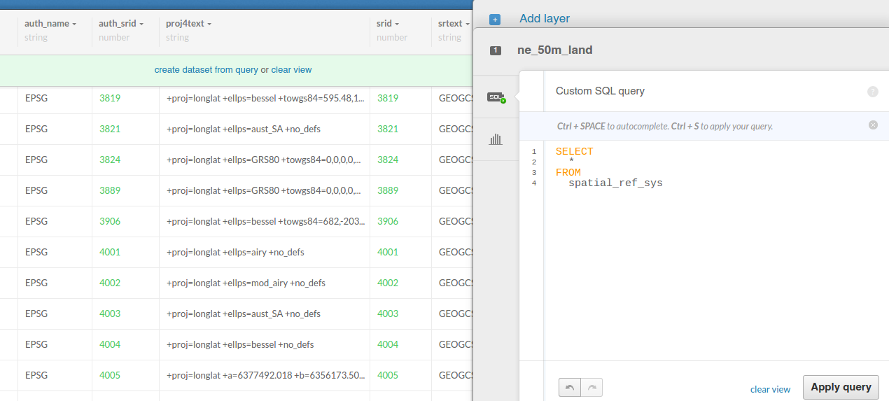
4. 2. Changing map projections
- Accessing the list of default projections available in CartoDB:
SELECT
  *
FROM
  spatial_ref_sys
- Accessing the occult the_geom_webmercator field:
SELECT
  the_geom_webmercator
FROM
  ne_50m_land
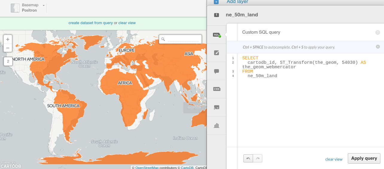
- World Robinson projection (ESPG:54030):
SELECT
  cartodb_id, ST_Transform(the_geom, 54030) AS the_geom_webmercator
FROM
  ne_50m_land
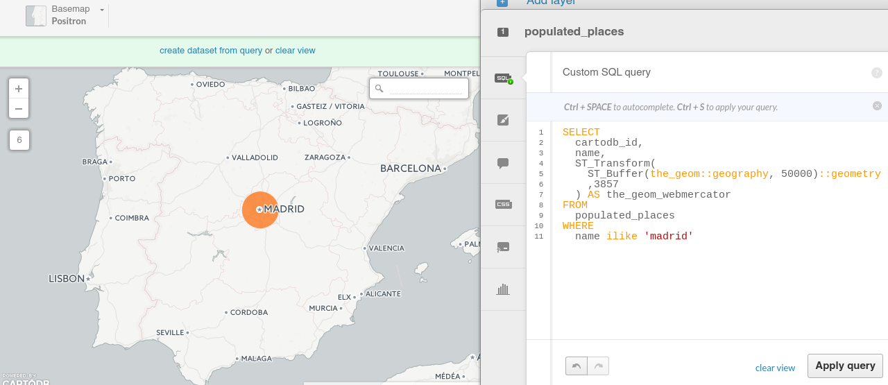
4. 3. Geoprocessing
- Create a buffer from points:
SELECT
  cartodb_id,
  name,
  ST_Transform(
    ST_Buffer(the_geom::geography, 50000)::geometry
    ,3857
  ) AS the_geom_webmercator
FROM
  populated_places
WHERE
  name ilike 'madrid'
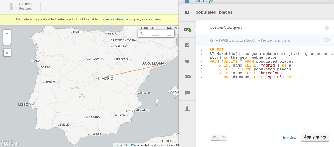
- Create a straight line between two points:
SELECT
  ST_MakeLine(a.the_geom_webmercator,b.the_geom_webmercator) as the_geom_webmercator
FROM (SELECT * FROM populated_places
    WHERE name ILIKE 'madrid') as a,
    (SELECT * FROM populated_places
    WHERE name ILIKE 'barcelona'AND adm0name ILIKE 'spain') as b
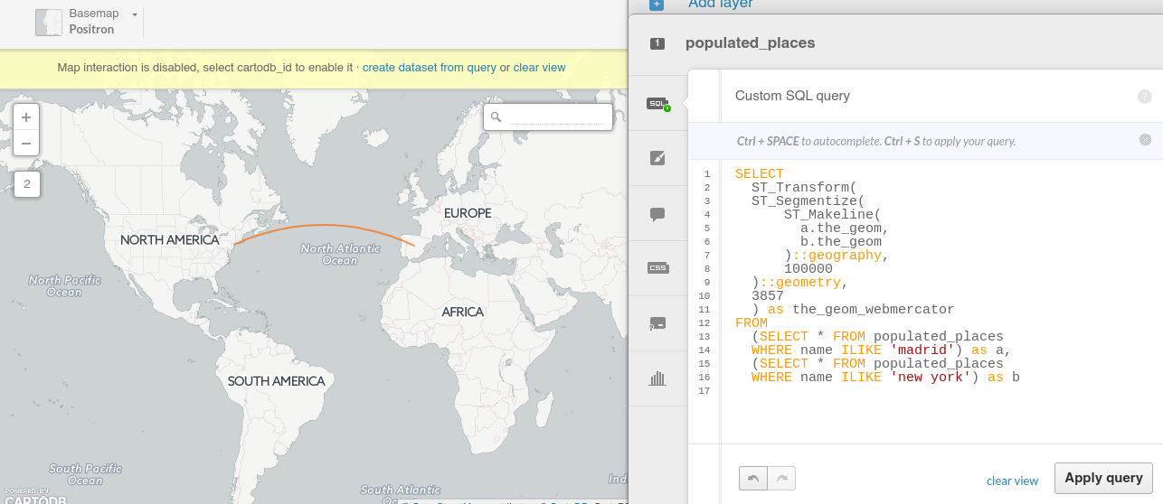
- Create a great circles between two points:
SELECT
  ST_Transform(
  ST_Segmentize(
      ST_Makeline(
        a.the_geom,
        b.the_geom
      )::geography,
      100000
  )::geometry,
  3857
  ) as the_geom_webmercator
FROM
  (SELECT * FROM populated_places
  WHERE name ILIKE 'madrid') as a,
  (SELECT * FROM populated_places
  WHERE name ILIKE 'new york') as b
5. Webmapping apps with CartoDB.js
5. 1. CartoDB.js
CartoDB.js is the JavaScript library that allows to create webmapping apps using CartoDB services quickly and efficiently. It’s built upon the following components:
- jQuery
- Underscore.js
- Backbone.js
- It can use either Google Maps API or Leaflet
5. 2. Examples
-
Add custom infowindow, infobox, tooltip & legend with with
createLayer(): example.