CartoDB Workshops : PostGIS & CartoCSS Intermediate Workshop

This intermediate workshop was given by Ramiro Aznar and Oriol Boix on June 18, 2016 at . As taught, it was 3h hours long.

Trainers:
- Ramiro Aznar · ramiroaznar@cartodb.com · @ramiroaznar
- Oriol Boix · oboix@cartodb.com · @oriolbx
Collaborators:
- Ernesto Martínez · ernesto@cartodb.com · @ernesmb
- Jorge Sanz · jorge@cartodb.com · @xurxosanz
June 18th 2016
PostGIS & CartoCSS Intermediate Workshop · GeoInquietos Madrid · Medialab-Prado

http://bit.ly/postgis-cartocss

workshop

The PostGIS worshops is based on the SIGLibre10 CartoDB Workshop. The CartoCSS workshop is also mainly based on the CartoDB Design Webinars conducted by Mamata Akella (@mamatakella) and Emilio García (@piensaenpixel):

Part 1 - Airport Traffic Map: slides & gist.
Part 2 - Migration Map: slides & gist.

Further questions and troubleshooting

Some questions could be already anwered at GIS Stack Exchange cartodb tag.
Email to support@cartodb.com.

Spatial Analysis with PostGIS
Cartographic Design with CartoCSS

1. Spatial Analysis with PostGIS

1. 0. Datasets

These are the datasets we are going to use on our workshop. You’ll find them all on our Data Library and fit way well on a free account.

Populated Places [ne_10m_populated_places_simple]: City and town points.
World Borders [world_borders]: World countries borders.
Land [ne_50m_land]: World emerged lands.
European countries [ne_adm0_europe]: European countries geometries.

1. 1. Working with projections

`geometry` vs. `geography`

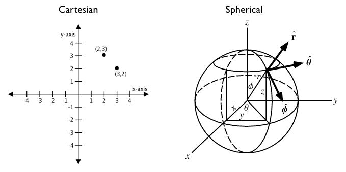
Geometry uses a cartesian plane to measure and store features (CRS units):

The basis for the PostGIS geometry type is a plane. The shortest path between two points on the plane is a straight line. That means calculations on geometries (areas, distances, lengths, intersections, etc) can be calculated using cartesian mathematics and straight line vectors.
Geography uses a sphere to measure and store features (Meters):

The basis for the PostGIS geography type is a sphere. The shortest path between two points on the sphere is a great circle arc. That means that calculations on geographies (areas, distances, lengths, intersections, etc) must be calculated on the sphere, using more complicated mathematics. For more accurate measurements, the calculations must take the actual spheroidal shape of the world into account, and the mathematics becomes very complicated indeed.

More about the geography type can be found here and here.

cart_vs_sph

LA-CDG

Source: Boundless Postgis intro

`the_geom` vs. `the_geom_webmercator`

the_geom EPSG:4326. Unprojected coordinates in decimal degrees (Lon/Lat). WGS84 Spheroid.
the_geom_webmercator EPSG:3857. UTM projected coordinates in mercator units. This is a conventional Coordinate Reference System, widely accepted as a ‘de facto’ standard in webmapping.

In CartoDB, the_geom_webmercator column is the one we see represented in the map. Know more about projections:

1. 2. Changing map projections

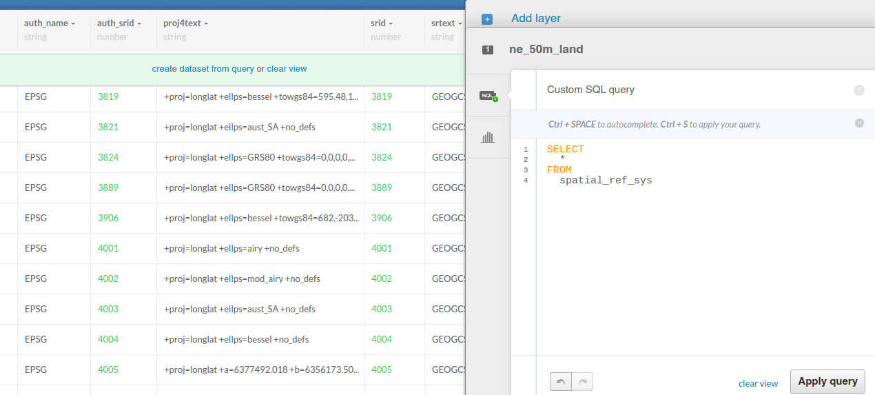
Accessing the list of default projections available in CartoDB:

SELECT
  *
FROM
  spatial_ref_sys

srid

Accessing the hidden the_geom_webmercator field:

SELECT
  the_geom_webmercator
FROM
  ne_50m_land

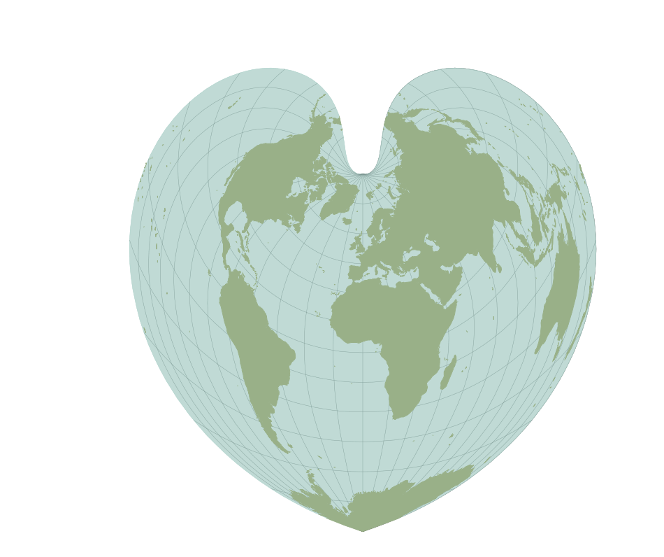
Adding World Robinson projection (ESPG:54030):

INSERT INTO spatial_ref_sys
  (srid, auth_name, auth_srid, proj4text, srtext) values (54030, 'EPSG', 54030,
'+proj=robin +datum=WGS84','PROJCS["World_Robinson",
    GEOGCS["GCS_WGS_1984",
        DATUM["WGS_1984",
            SPHEROID["WGS_1984",6378137,298.257223563]],
        PRIMEM["Greenwich",0],
        UNIT["Degree",0.017453292519943295]],
    PROJECTION["Robinson"],
    PARAMETER["False_Easting",0],
    PARAMETER["False_Northing",0],
    PARAMETER["Central_Meridian",0],
    UNIT["Meter",1],
    AUTHORITY["EPSG","54030"]]');

ST_Transform()

SELECT
  cartodb_id, ST_Transform(the_geom, 54030) AS the_geom_webmercator
FROM
  ne_50m_land

robinson

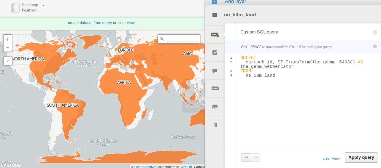
About ST_Transform.

1. 3 Geometric relations

Equals: ST_Equals
Disjoint: ST_Disjoint
Intersects: ST_Intersects
Touches: ST_Touches
Crosses: ST_Crosses
Within: ST_Within
Contains: ST_Contains
Overlaps: ST_Overlaps

Examples:

spatialrelations

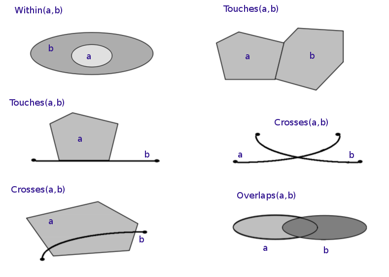
Source: Wikipedia examples of spatial relations

*Important: The geometric relations are very strict, make sure that the geometries that you will use are valid. Use the valid functions of PostGIS to check if the geometries are valid or not.

About ST_isValid,ST_MakeValid,ST_isValidReason,ST_IsValidDetail.

Get the number of points inside a polygon

Using GROUP BY:

SELECT
  e.cartodb_id,
  e.admin,
  e.the_geom_webmercator,
  count(*) AS pp_count,
  sum(p.pop_max) as sum_pop
FROM
  ne_adm0_europe e
JOIN
  ne_10m_populated_places_simple p
ON
  ST_Intersects(p.the_geom, e.the_geom)
GROUP BY
  e.cartodb_id

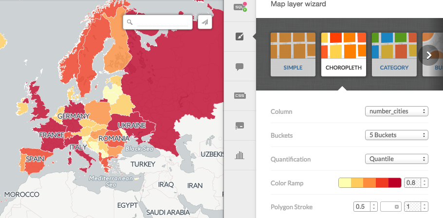
Using LATERAL:

SELECT
  a.cartodb_id,
  a.admin AS name,
  a.the_geom_webmercator,
  counts.number_cities,
  to_char(counts.sum_pop,'999,999,999') as sum_pop --decimal separator
FROM
  ne_adm0_europe a
CROSS JOIN LATERAL
  (
    SELECT
      count(*) as number_cities,
      sum(pop_max) as sum_pop
    FROM
      ne_10m_populated_places_simple b
    WHERE
      ST_Intersects(a.the_geom, b.the_geom)
  ) AS counts

About Lateral JOIN

intersects

1. 4 Proximity analysis

ST_Distance

SELECT b.name, st_distance(a.the_geom_webmercator,b.the_geom_webmercator) as distancia
FROM
  ne_10m_populated_places_simple a,
  ne_10m_populated_places_simple b
WHERE
ST_distance(a.the_geom_webmercator,b.the_geom_webmercator) < 300000
  AND a.name = 'Madrid'
  AND a.cartodb_id != b.cartodb_id
ORDER BY st_distance(a.the_geom_webmercator,b.the_geom_webmercator)

Execution time: 8.344 ms

About ST_Distance.

ST_Expand + ST_Distance

SELECT b.name, st_distance(a.the_geom_webmercator,b.the_geom_webmercator) as distancia
FROM
  ne_10m_populated_places_simple a,
  ne_10m_populated_places_simple b
WHERE
ST_Expand(a.the_geom_webmercator,300000) && b.the_geom_webmercator
AND
ST_distance(a.the_geom_webmercator,b.the_geom_webmercator) < 300000
  AND a.name = 'Madrid'
  AND a.cartodb_id != b.cartodb_id
ORDER BY st_distance(a.the_geom_webmercator,b.the_geom_webmercator)

Execution time: 3.452 ms

About ST_Expand.

ST_DWithin

SELECT b.name,st_distance(a.the_geom_webmercator,b.the_geom_webmercator) as distancia
FROM
  ne_10m_populated_places_simple a,
  ne_10m_populated_places_simple b
WHERE
ST_DWithin(a.the_geom_webmercator,b.the_geom_webmercator,300000)
  AND a.name = 'Madrid'
  AND a.cartodb_id != b.cartodb_id
ORDER BY st_distance(a.the_geom_webmercator,b.the_geom_webmercator)

Execution time: 2.006 ms

About ST_DWithin.

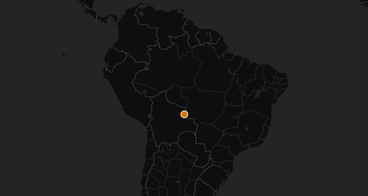
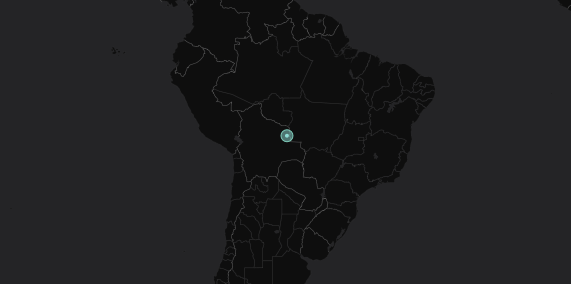
1. 5 Geoprocessing

Create a buffer from points:

SELECT
  cartodb_id,
  name,
  ST_Transform(
    ST_Buffer(the_geom::geography, 50000)::geometry
    ,3857
  ) AS the_geom_webmercator
FROM
  ne_10m_populated_places_simple
WHERE
  name ilike 'madrid'

buffer

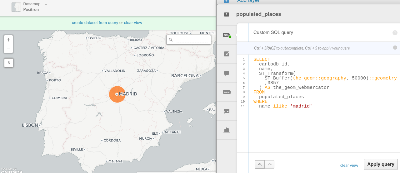
About ST_Buffer.

Note: try to compute a Buffer on a place with high latitude and check the difference between using directly the_geomwebmecator and the_geom::geography —

Get the difference between two geometries:

SELECT
  a.cartodb_id,
    ST_Difference(
        a.the_geom_webmercator,
        b.the_geom_webmercator
  ) AS the_geom_webmercator
FROM
  ne_50m_land a,
  ne_adm0_europe b
WHERE
  b.adm0_a3 like 'ESP'

difference

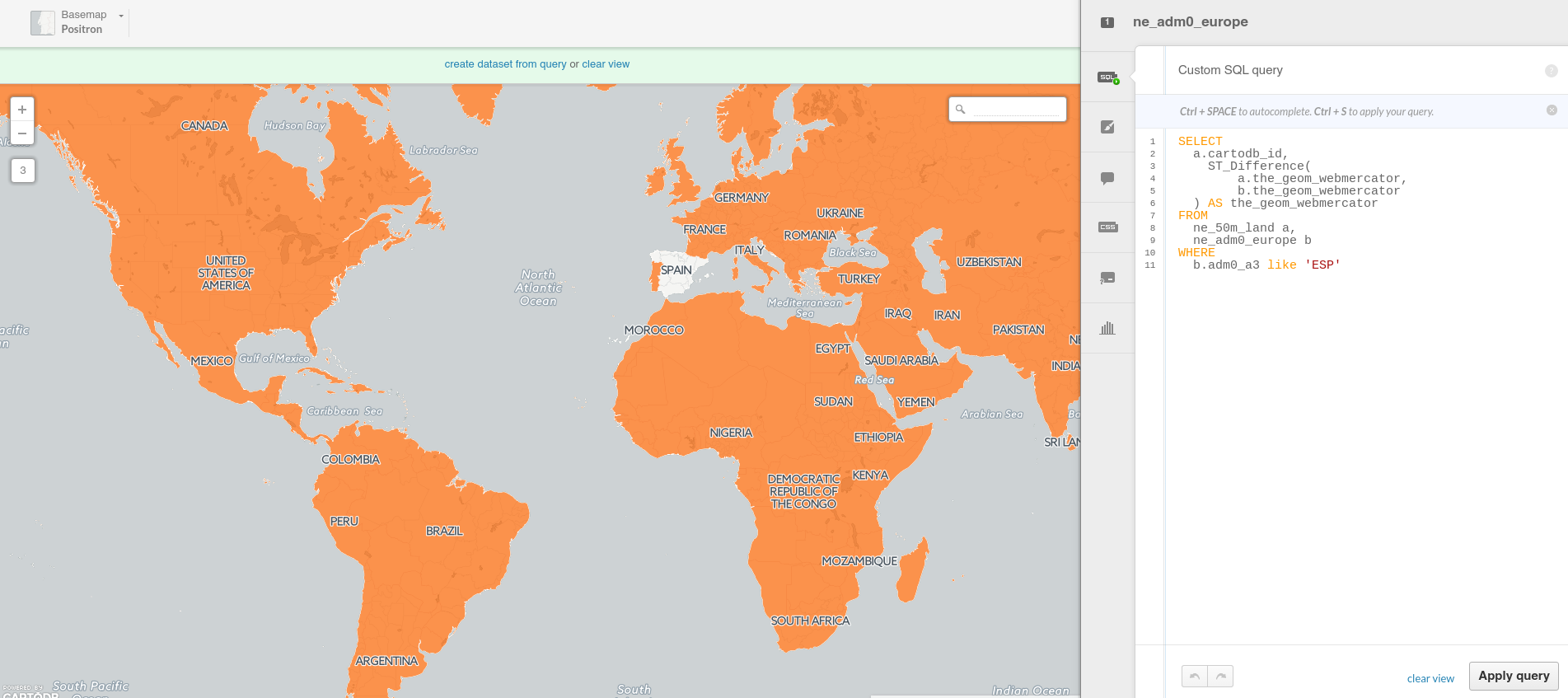
About ST_Difference.

Create a straight line between two points:

SELECT
  ST_MakeLine(a.the_geom_webmercator,b.the_geom_webmercator) as the_geom_webmercator
FROM (SELECT * FROM ne_10m_populated_places_simple
    WHERE name ILIKE 'madrid') as a,
    (SELECT * FROM ne_10m_populated_places_simple
    WHERE name ILIKE 'barcelona'AND adm0name ILIKE 'spain') as b

lines

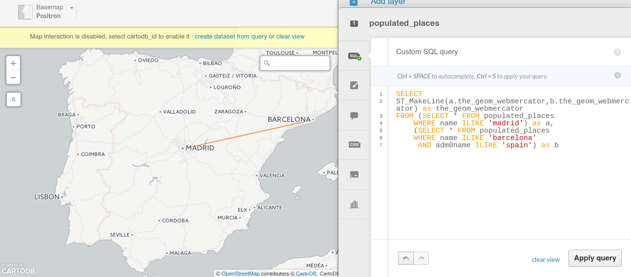
About ST_MakeLine.

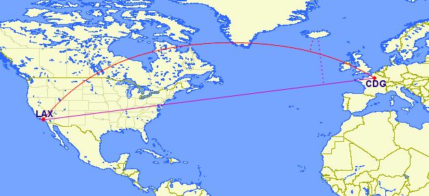
Create great circles between two points:

SELECT
  ST_Transform(
  ST_Segmentize(
      ST_Makeline(
        a.the_geom,
        b.the_geom
      )::geography,
      100000
  )::geometry,
  3857
  ) as the_geom_webmercator
FROM
  (SELECT * FROM ne_10m_populated_places_simple
  WHERE name ILIKE 'madrid') as a,
  (SELECT * FROM ne_10m_populated_places_simple
  WHERE name ILIKE 'new york') as b

greatcircles

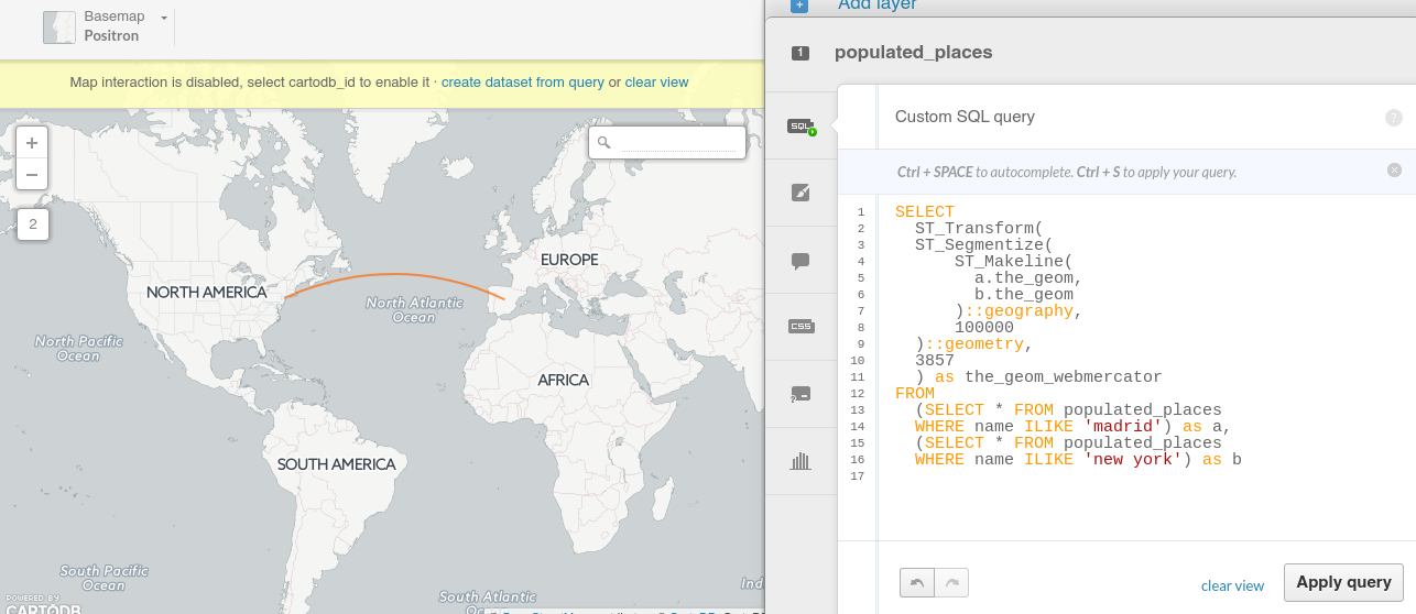
About Great Circles.

Generating Grids with CDB functions

Rectangular grid

SELECT
  row_number() over () as cartodb_id,
  CDB_RectangleGrid(
    ST_Buffer(the_geom_webmercator,125000),
  250000,
  250000
  ) AS the_geom_webmercator
FROM
  ne_adm0_europe
WHERE
  adm0_a3 IN ('ITA','GBR')

ADD IMAGE

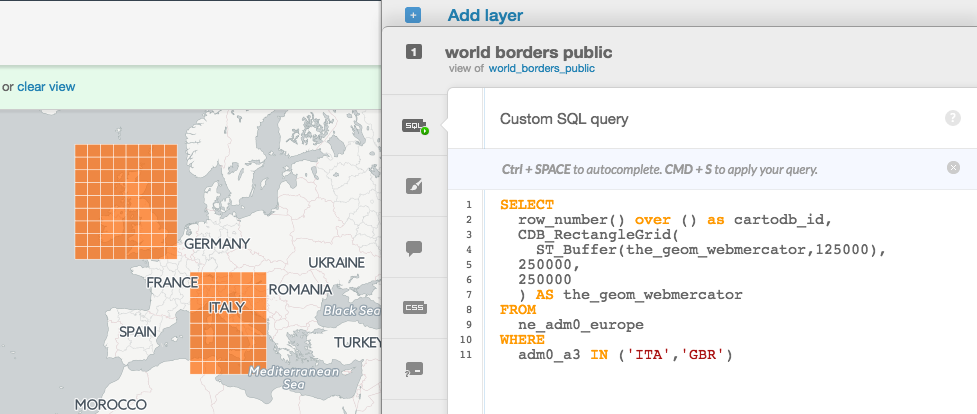
About CDB_RectangleGrid

Adaptative Hexagonal grid

WITH grid AS
(SELECT
  row_number() over () as cartodb_id,
  CDB_HexagonGrid(
    ST_Buffer(the_geom_webmercator, 100000),
    100000
  ) AS the_geom_webmercator
FROM
  ne_adm0_europe
WHERE
  adm0_a3 IN ('ESP','ITA'))

SELECT
  grid.the_geom_webmercator,
  grid.cartodb_id
FROM
  grid, ne_adm0_europe a
WHERE
    ST_intersects(grid.the_geom_webmercator, a.the_geom_webmercator)
  AND a.adm0_a3 IN ('ESP','ITA')

ADD IMAGE

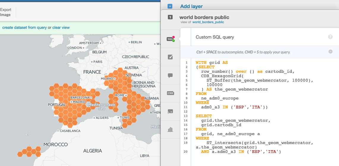
About CDB_HexagonGrid

2. Cartographic Design with CartoCSS

2. 1. (Some) Design Principles

Slides

bone

2. 2. Styling with CartoCSS

2. 2. 1. CartoCSS best practices

While there are many ways to apply the same visual effects with CartoCSS properties, this section describes the most efficient and intuitive methods for structuring your CartoCSS syntax.

You can apply CartoCSS properties to the overall map style, or to specific map symbolizers (such as markers and points). Sometimes, applying properties to a symbolizer is not the most effective workflow for enhancing your overall map style. Other times, applying a style to the overall map is not rendered if there is no default value defined, and thus, not needed. For example, see how composite operations can be used for color blending, based on style or symbolizer.

When applying CartoCSS syntax, it helps to understand how values are applied to your map:

The source is where the style is applied (either as a value or as a symbolizer property)
The destination is the effect on the rest of the map, underneath the source
Any layers that appear above the source are unaffected by the applied style and are rendered normally
Typically, you apply CartoCSS properties to different layers on a map. You can add multiple styles and values for each layer
Alternatively, you can apply CartoCSS by nesting categories and values. Categories contain multiple values listed under the same, single category using brackets { }. This enables you visualize all of the styling elements applied to the overall map or to individual symbolizers, and avoid adding any redundant or unnecessary parameters. This is the suggested method if you are applying styles to a multi-scale map.

Note: Be mindful when applying styles to a map with multiple layers. Instead of applying an overall style to each map layer, apply the style to one layer on the map using this nested structure. For example, suppose you have a map with four layers, you can define zoom dependent styling as a nested value in one map layer. You do not have to go through each layer of the map to apply a zoom style. Using the nested structure allows you to apply all of the styling inside the brackets { }. This is a more efficient method of applying overall map styling.

Search in the Data Library the continents dataset, connect it and disable the sync connection. Then run the following SQL query, visualize it and rename the map as continents_centroids:

SELECT 
  cartodb_id,
  name as continent,
  st_transform(st_centroid(the_geom),3857) as the_geom_webmercator
FROM 
  continents

Note how the CartoCSS syntax is structured:

CartoCSS syntax structured by @ values

value

@africa: #A6CEE3;
@antarctica: #1F78B4;
@asia: #B2DF8A;
@australia: #33A02C;
@europe: #FB9A99;
@northamerica: #E31A1C;
@oceania: #FDBF6F;
@southamerica:#FF7F00; 

#continents {
  marker-fill-opacity: 0.9;
  marker-line-color: #FFF;
  marker-line-width: 1;
  marker-width: 10;
  marker-allow-overlap: true;

  [continent="Africa"] {
   marker-fill: @africa;
  }
  [continent="Antarctica"] {
    marker-fill: @antarctica;
  }
  [continent="Asia"] {
    marker-fill: @asia;
  }
  [continent="Australia"] {
    marker-fill: @australia;
  }
  [continent="Europe"] {
    marker-fill: @europe;
  }
  [continent="North America"] {
    marker-fill: @northamerica;
  }
  [continent="Oceania"] {
    marker-fill: @oceania;
  }
  [continent="South America"] {
    marker-fill: @southamerica;
  }
}

CartoCSS syntax structured by styling over an already styled feature

replicating

#continents{
      marker-fill-opacity: 1;
      marker-line-color: #7fcdbb;
      marker-line-width: 1;
      marker-line-opacity: 0;
      marker-placement: point;
      marker-type: ellipse;
      marker-width: 4;
      marker-fill: #91e1d8;
      marker-allow-overlap: true;
    }
  #continets::point{
      marker-fill-opacity: 0.5;
      marker-line-color: #7fcdbb;
      marker-line-width: 1;
      marker-line-opacity: 1;
      marker-placement: point;
      marker-type: ellipse;
      marker-width: 12;
      marker-fill: #91e1d8;
      marker-allow-overlap: true;
    }

CartoCSS syntax structure to style layer labels

labels

Map {
  buffer-size: 2000; /* Ensures that labels crossing tile boundaries are equally rendered in each tile. */
    }
#continents::labels {
  text-name: [continent];
  text-face-name: "Open Sans Bold";
  text-size: 12;
  text-fill: #FFFFFF;
  text-halo-fill: fadeout(#000000, 30%);
  text-halo-radius: 2;
  text-allow-overlap: true;
  text-placement: point;
  text-placement-type: simple;
  text-dy: 10;
    }

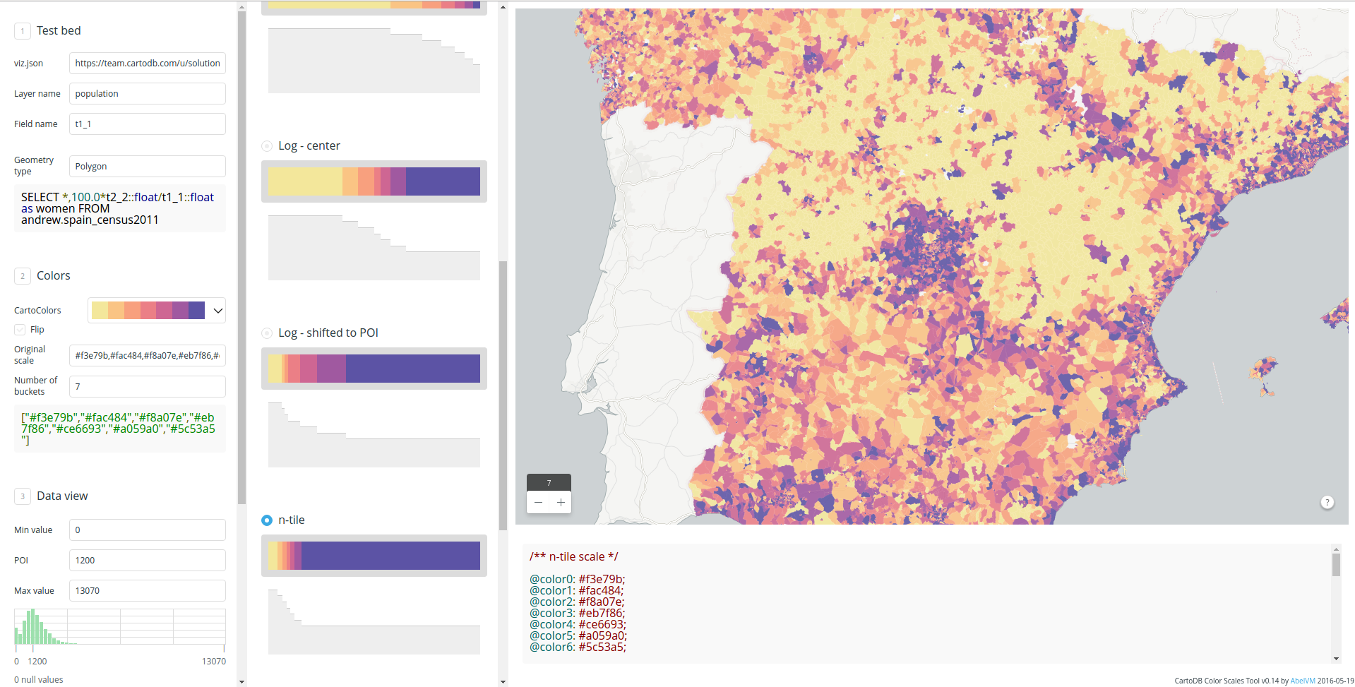
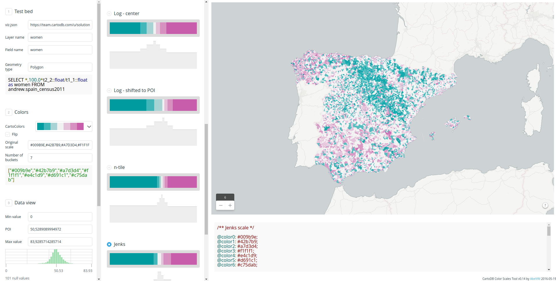
2. 2. 2. CartoColors

Labs-ColorScales, an app to obtain CartoCSS palettes from a viz.json, a layer and a numeric field.

Sequential Palettes

sequential

Qualitative Paletters

Sequential + Qualitative Paletters

Diverging palettes

diverging

2. 2. 3. Turbo-Carto

Next-Gen Styling for Data-Driven Maps, CartoCSS is alive! Bl.ock

2. 3. Let’s get mapping!

2. 3. 1. Make a custom basemap…

First, we will create a simple basemap that we can use to display the airport traffic information on top of.

Add the data

From your Maps dashboard, click on NEW MAP.
In the Add datasets dialogue, search for “world borders” to find the World Borders (High Definition) dataset available in the CartoDB Library.
Once located, click to highlight, and then click CREATE MAP which will sync the layer to your account from the CartoDB Library and also add it to our map.

Style the background

The default basemap is Positron to change that, let’s change the background color of the map. In the Editor choose “Change basemap” and change the default color to #2e3c43.

Style the countries

To continue with the subtle theme for our basemap, we’ll style the countries so they sit nicely with the background color of the map. First, let’s rename the layer to “Basemap”. Next, we’ll open the styling Wizard and change the following properties:

/** Basemap Style */

#basemap{
polygon-fill: #FFFFFF;
polygon-opacity: 0.5;
line-color: #FFF;
line-width: 0.25;
line-opacity: 0.1;
}

Give our Map a Title

Double click on the title and change it to “Airport Traffic”.

2. 3. 2. …and then an airport traffic map!

Add Layer with the airport points dataset: - Click on “Add Layer”. - Click on “Connect dataset”. - Copy this URL: https://cartotraining.cartodb.com/api/v2/sql?q=select%20*%20from%20cartotraining.airport_traffic_points&format=csv - Submit!
Rename as to Airports Points
Style point layer:

#airport_points{
marker-fill-opacity: 0.6;
marker-line-color: #3E7BB6;
marker-line-width: 0.20;
marker-line-opacity: 0;
marker-placement: point;
marker-multi-policy: largest;
marker-type: ellipse;
marker-fill: #FFFFFF;
marker-allow-overlap: true;
marker-clip: false;
  }

For more context we are going to style this layer depends the number of users:

      #airport_points [ users <= 249143] {
         marker-width: 6.0;
      }
      #airport_points [ users <= 35019] {
         marker-width: 5.4;
      }
      #airport_points [ users <= 22640] {
         marker-width: 4.9;
      }
      #airport_points [ users <= 16512] {
         marker-width: 4.3;
      }
      #airport_points [ users <= 12334] {
         marker-width: 3.8;
      }
      #airport_points [ users <= 9051.5] {
         marker-width: 3.2;
      }
      #airport_points [ users <= 6472] {
         marker-width: 2.7;
      }
      #airport_points [ users <= 4445] {
         marker-width: 2.1;
      }
      #airport_points [ users <= 2752] {
         marker-width: 1.6;
      }
      #airport_points [ users <= 1266] {
         marker-width: 1.0;
      }

Add Layer with the airport routes dataset: - Click on “Add Layer”. - Click on “Connect dataset”. - Copy this URL: https://cartotraining.cartodb.com/api/v2/sql?q=select%20*%20from%20cartotraining.airport_traffic_routes&format=csv - Submit!
Rename as Airports Routes

We style the lines:

   #airport_routes {
     polygon-opacity: 0;
     line-color: #5CA2D1;
     line-width: .25;
     line-opacity: 1;
   }

If you like we could style the line depends the number of users:

   #airport_routes [ users <= 229457] {
     line-opacity: 0.40;
   }
   #airport_routes [ users <= 26186] {
     line-opacity: 0.35;
   }
   #airport_routes [ users <= 15551] {
     line-opacity: 0.30;
   }
   #airport_routes [ users <= 10161] {
     line-opacity: 0.25;
   }
   #airport_routes [ users <= 6115] {
     line-opacity: 0.20;
   }
   #airport_routes [ users <= 3320] {
     line-opacity: 0.15;
   }
   #airport_routes [ users <= 1245] {
     line-opacity: .1;
   }

Change the order of the layers, put the airports point on the top
Add title and customize legends

Publish the final map

You can take a look this blog post about how to draw great circles instead of lines:

CartoDB Workshops Materials for Teaching Maps

PostGIS & CartoCSS Intermediate Workshop