SIGLibre10 CartoDB Workshop
- Trainers:
- Jorge Sanz · jorge@cartodb.com · @xurxosanz
- Oriol Boix · oboix@cartodb.com · @oriolbx
- Collaborators:
- Ernesto Martínez · ernesto@cartodb.com · @ernesmb
- Ramiro Aznar · ramiroaznar@cartodb.com · @ramiroaznar
- May 28th 2016
- 10as Jornadas de SIG Libre
Intro Slides
http://cartodb.github.io/training/intermediate/siglibre10-workshop.html
Further questions and troubleshooting
- GIS Stack Exchange
cartodbtag - email to support@cartodb.com
Contents
- Importing datasets
- Getting your data ready
- Making a map
- Going spatial with PostGIS
- Webmapping apps with CartoDB.js
0. Before we start…
CartoDB as a platform:
- Import API allows to upload new data to CartoDB.
- SQL API allows to interact with CartoDB tables. Query and modify CartoDB tables.
- Maps API allows to visualize the underlying data.
The CartoDB Editor is a client of the platform
1. Importing datasets
1.1 Supported Geospatial Data Files
CartoDB supports the following geospatial data formats to upload vector data*:
ShapefileKMLKMZGeoJSON*CSVSpreadsheetsGPXOSM
Importing different geometry types in the same layer or in a FeatureCollection element (GeoJSON) is not supported. More detailed information here.
[*] More detailed information about GeoJSON format here, here and here.
1.2 Common importing errors
- Dataset too large:
- File size limit: 150 Mb (free).
- Import row limit: 500,000 rows (free).
- Solution: split your dataset into smaller ones, import them into CartoDB and merge them.
- Malformed CSV:
- Solution: check termination lines, header…
- Encoding:
- Solution:
Save with Encoding>UTF-8 with BOMin Sublime Text, any other decent text editor or iconv.
- Solution:
- Shapefile missing files:
- Missing any of the following files within the compressed file will produce an importing error:
.shp: contains the geometry. REQUIRED..shx: contains the shape index. REQUIRED..prj: contains the projection. REQUIRED..dbf: contains the attributes. REQUIRED.
- Other auxiliary files such as
.sbn,.sbxor.shp.xmlare not REQUIRED. - Solution: make sure to add all required files.
- Missing any of the following files within the compressed file will produce an importing error:
- Duplicated id fields:
- Solution: check your dataset, remove or rename fields containing the
idkeyword.
- Solution: check your dataset, remove or rename fields containing the
- Format not supported:
- URLs -that are not points to a file- are not supported by CartoDB.
- Solution: check for missing url parameters or download the file into your local machine, import it into CartoDB.
- MAYUS extensions not supported:
example.CSVis not supported by CartoDB.- Solution: rename the file.
- Non supported SRID:
- Solution: try to reproject your resources locally to a well known projection like
EPSG:4326,EPSG:3857,EPSG:25830and so on.
- Solution: try to reproject your resources locally to a well known projection like
Other importing errors and their codes can be found here.
2. Getting your data ready
2.1 Geocoding
If you have a column with longitude coordinates and another with latitude coordinates, CartoDB will automatically detect and covert values into the_geom. If this is not the case, CartoDB can help you by turning the named places into best guess of latitude-longitude coordinates:
- By Lon/Lat Columns.
- By City Names.
- By Admin. Regions.
- By Postal Codes.
- By IP Addresses.
- By Street Addresses.
Know more about geocoding in CartoDB:
- In this tutorial.
- In our Location Data Services website.
- In our documentation.
2.2 Datasets
These are the datasets we are going to use on our workshop. You’ll find them all on our Data Library and fit way well on a free account.
- Populated Places [
ne_10m_populated_places_simple]: City and town points. - World Borders [
world_borders]: World countries borders. - Land [
ne_50m_land]: World emerged lands. - European countries [
ne_adm0_europe]: European countries geometries.
2.3 Simple SQL operations
Selecting all columns:
SELECT
  *
FROM
  ne_10m_populated_places_simple;
Selecting some columns:
SELECT
  cartodb_id,
  name as city,
  adm1name as region,
  adm0name as country,
  pop_max,
  pop_min
FROM
  ne_10m_populated_places_simple
Selecting distinct values:
SELECT DISTINCT
  adm0name as country
FROM
  ne_10m_populated_places_simple
2.4 Filtering
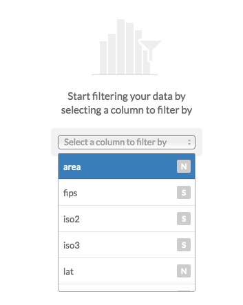
Filtering numeric fields:
SELECT
  *
FROM
  ne_10m_populated_places_simple
WHERE
  pop_max > 5000000;
Filtering character fields:
SELECT
  *
FROM
  ne_10m_populated_places_simple
WHERE
  adm0name ilike 'spain'
Filtering a range:
SELECT
  *
FROM
  ne_10m_populated_places_simple
WHERE
  name in ('Madrid', 'Barcelona')
AND
  adm0name ilike 'spain'
Combining character and numeric filters:
SELECT
  *
FROM
  ne_10m_populated_places_simple
WHERE
  name in ('Madrid', 'Barcelona')
AND
  adm0name ilike 'spain'
AND
  pop_max > 5000000
2.5 Others:
Selecting aggregated values:
count
SELECT
  count(*) as total_rows
FROM
  ne_10m_populated_places_simple
sum
SELECT
  sum(pop_max) as total_pop_spain
FROM
  ne_10m_populated_places_simple
WHERE
  adm0name ilike 'spain'
avg
SELECT
  avg(pop_max) as avg_pop_spain
FROM
  ne_10m_populated_places_simple
WHERE
  adm0name ilike 'spain'
Ordering results:
SELECT
  cartodb_id,
  name as city,
  adm1name as region,
  adm0name as country,
  pop_max
FROM
  ne_10m_populated_places_simple
WHERE
  adm0name ilike 'spain'
ORDER BY
  pop_max DESC
Limiting results:
SELECT
  cartodb_id,
  name as city,
  adm1name as region,
  adm0name as country,
  pop_max
FROM
  ne_10m_populated_places_simple
WHERE
  adm0name ilike 'spain'
ORDER BY
  pop_max DESC
LIMIT 10
3. Making our first map
3.0 Before we start…
CartoDB makes maps using SQL queries, not tables!
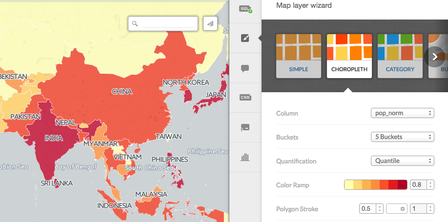
3.1 Wizard
Analyzing your dataset… In some cases, when you connect a dataset and click on the MAP VIEW for the first time, the Analyzing dataset dialog appears. This analytical tool analyzes the data in each column, predicts how to visualize this data, and offers you snapshots of the visualized maps. You can select one of the possible map styles, or ignore the analyzing dataset suggestions.
- Simple Map
- Cluster Map
- Category Map
- Bubble Map
- Torque Map
- Heatmap Map
- Torque Cat Map
- Intensity Map
- Density Map
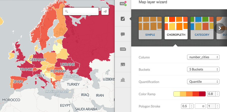
- Choropleth Map:
Before making a choropleth map, we need to normalize our target column. For that, we need to divide the population by the area. More about what that ::geography means later.
SELECT
  wb.*,
  pop2005/(ST_Area(the_geom::geography)/1000000) AS pop_norm
FROM
  world_borders wb
Click on ‘create new dataset from query’.
Rename the new dataset to world_borders_norm
Know more about chosing the right map to make here.
3.2 Styles
The last link in the website referenced above is a great discussion about the different maps CartoDB allows to create.
Simple Map:
/** simple visualization */

#layer{
  polygon-fill: #FF6600;
  polygon-opacity: 0.7;
  line-color: #FFF;
  line-width: 0.5;
  line-opacity: 1;
}
Choropleth Map:
/** choropleth visualization */

#layer{
  polygon-fill: #FFFFB2;
  polygon-opacity: 0.8;
  line-color: #FFF;
  line-width: 0.5;
  line-opacity: 1;
}
#layer [ pop_norm <= 247992435.530086] {
   polygon-fill: #B10026;
}
#layer [ pop_norm <= 4086677.23673585] {
   polygon-fill: #E31A1C;
}
#layer [ pop_norm <= 1538732.3943662] {
   polygon-fill: #FC4E2A;
}
#layer [ pop_norm <= 923491.374542489] {
   polygon-fill: #FD8D3C;
}
#layer [ pop_norm <= 616975.331234902] {
   polygon-fill: #FEB24C;
}
#layer [ pop_norm <= 326396.192958792] {
   polygon-fill: #FED976;
}
#layer [ pop_norm <= 95044.5589361554] {
   polygon-fill: #FFFFB2;
}
Proportional symbols map
Take a look on this excellent blog post by Mamata Akella_ regarding how to produce proportional symbols maps. The easiest ones being buble maps since it’s directly supported by CartoDB wizards. The other type, the graduated symbols where you compute the radius of the symbol to be used later on the CartoCSS section needs a bit of SQL computation but nothing hard.
WITH aux AS(
  SELECT
    max(pop2005) AS max_pop
  FROM
    world_borders
  )
SELECT
  cartodb_id,
  pop2005,
  ST_Centroid(the_geom_webmercator) AS the_geom_webmercator,
  5+30*sqrt(pop2005)/sqrt(aux.max_pop) AS size
FROM
  world_borders,
  aux
#layer{
  marker-fill-opacity: 0.8;
  marker-line-color: #FFF;
  marker-line-width: 1;
  marker-line-opacity: 1;
  marker-width: [size];
  marker-fill: #FF9900;
  marker-allow-overlap: true;
}
Two-variable CartoCSS
It’s common practice to use two visual variables, typically color and size to represent one or two variables. To do this easily using CartoDB wizards you start for example with a coropleth map, copy on a separate text file the CartoCSS section where the field is used to color the geometries, then change the wizard to the bubble map and paste the previous code so instead of one color bubbles you get both variables styled.
- SQL
WITH aux AS
  (
  SELECT
    max (pop_max) AS max_population
  FROM
    ne_10m_populated_places_simple
  )
SELECT
  a.*,
  (pop_max*100)/aux.max_population AS pop_norm
FROM
  ne_10m_populated_places_simple a,
  aux
- CartoCSS
/** bubble visualization */
#ne_10m_populated_places_simple [ pop_norm < 100] {
   marker-width: 25.0;
}
#ne_10m_populated_places_simple [ pop_norm < 90] {
   marker-width: 23.3;
}
#ne_10m_populated_places_simple [ pop_norm < 80] {
   marker-width: 21.7;
}
#ne_10m_populated_places_simple [ pop_norm < 70] {
   marker-width: 20.0;
}
#ne_10m_populated_places_simple [ pop_norm < 60] {
   marker-width: 18.3;
}
#ne_10m_populated_places_simple [ pop_norm < 50] {
   marker-width: 16.7;
}
#ne_10m_populated_places_simple [ pop_norm < 40 {
   marker-width: 15.0;
}
#ne_10m_populated_places_simple [ pop_norm < 30] {
   marker-width: 13.3;
}
#ne_10m_populated_places_simple [ pop_norm < 20] {
   marker-width: 11.7;
}
#ne_10m_populated_places_simple [ pop_norm < 10] {
   marker-width: 10.0;
}

/** category visualization */
#ne_10m_populated_places_simple[megacity=0] {
   marker-fill: #FF9900;
}
#ne_10m_populated_places_simple[megacity=1] {
   marker-fill: #B81609;
}
A combination of the two methods above
- SQL
WITH aux AS(
  SELECT
    max(pop2005) AS max_pop
  FROM
    world_borders_norm
  )
SELECT
  cartodb_id,
  pop2005,
  ST_Centroid(the_geom_webmercator) AS the_geom_webmercator,
  5+30*sqrt(pop2005)/sqrt(aux.max_pop) AS size
FROM
  world_borders_norm,
  aux
- CartoCSS
#layer{
  marker-fill-opacity: 0.8;
  marker-line-color: #FFF;
  marker-line-width: 1;
  marker-line-opacity: 1;
  marker-width: [size];
  marker-fill: #FF9900;
  marker-allow-overlap: true;
}

#world_borders [ pop_norm <= 247992435.530086] {
   polygon-fill: #B10026;
}
#world_borders [ pop_norm <= 4086677.23673585] {
   polygon-fill: #E31A1C;
}
#world_borders [ pop_norm <= 1538732.3943662] {
   polygon-fill: #FC4E2A;
}
#world_borders [ pop_norm <= 923491.374542489] {
   polygon-fill: #FD8D3C;
}
#world_borders [ pop_norm <= 616975.331234902] {
   polygon-fill: #FEB24C;
}
#world_borders [ pop_norm <= 326396.192958792] {
   polygon-fill: #FED976;
}
#world_borders [ pop_norm <= 95044.5589361554] {
   polygon-fill: #FFFFB2;
}
Know more about CartoCSS with our documentation.
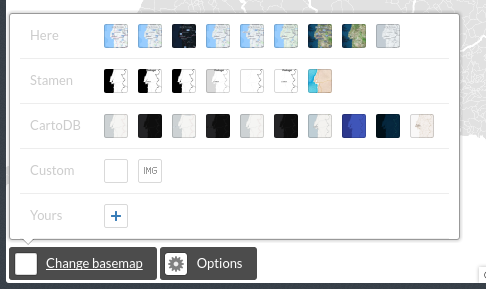
3.3 Other elements
Basemaps:
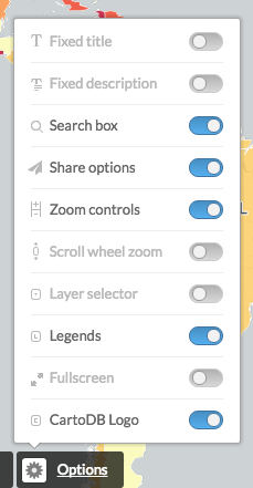
Options:
Legend:
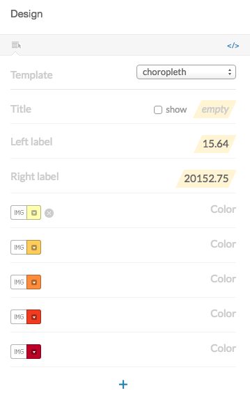
By clicking on the </> icon, you would see and edit the source HTML code
<div class='cartodb-legend choropleth'>
<div class="legend-title">Total Population</div>
<ul>
	<li class="min">
		95044.56
	</li>
	<li class="max">
		247992435.53
	</li>
	<li class="graph count_441">
	<div class="colors">
	<div class="quartile" style="background-color:#FFFFB2"></div>
	<div class="quartile" style="background-color:#FED976"></div>
	<div class="quartile" style="background-color:#FEB24C"></div>
	<div class="quartile" style="background-color:#FD8D3C"></div>
	<div class="quartile" style="background-color:#FC4E2A"></div>
	<div class="quartile" style="background-color:#E31A1C"></div>
	<div class="quartile" style="background-color:#B10026"></div>
	</div>
	</li>
</ul>
</div>
Labels:
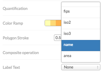
Selecting a field in the wizard will produce the following CartoCSS code to render the labels.
#world_borders::labels {
  text-name: [name];
  text-face-name: 'DejaVu Sans Book';
  text-size: 10;
  text-label-position-tolerance: 10;
  text-fill: #000;
  text-halo-fill: #FFF;
  text-halo-radius: 1;
  text-dy: -10;
  text-allow-overlap: true;
  text-placement: point;
  text-placement-type: simple;
}
This also shows an important concept for CartoCSS. you can specify more than one rendering pass for your features. This means that using the #layername::passname notation you can render more than one symbol on your features. One typical example of this feature is to render lines with more than one symbol.
#layer::background{
  line-width: 10;
  line-color: red;
}
#layer::foreground{
  line-width: 5;
  line-color: white;
}
On the above simplified CartoCSS example we use the same layer for a red background, 10 pixels widh, and then on top of it a white 5 pixels symbol.
Zoom based styling
The last feature we are going to cover here about CartoCSS is zoom based styling. In the same way we can do thematic maps specifying new rules for a set of features, we can also apply different rules for different zoom levels of our map. This means we can for example show the labels only between some zoom levels or increase the width of our line features when we are on high zooms. This can be achieved exactly in the same way we did with our choropleth map. So a possible
@1 : #F11810;


#ne_10m_populated_places_simple{
  marker-fill-opacity: 0.9;
  marker-line-color: lighten(@1,30);
  marker-line-width: 1;
  marker-line-opacity: 1;
  marker-placement: point;
  marker-multi-policy: largest;
  marker-type: ellipse;
  marker-fill: @1;
  marker-allow-overlap: true;
  marker-clip: false;

  [zoom < 3][pop_norm <= 30]{
   marker-fill-opacity:0;
   marker-line-opacity:0;
  }
  [zoom < 5][pop_norm <= 10]{
   marker-fill-opacity:0;
   marker-line-opacity:0;
  }
  [zoom < 7][pop_norm <= 1]{
   marker-fill-opacity:0;
   marker-line-opacity:0;
  }
}

/* normal buble classification here */
On the example above check how we nest inside the normal CartoCSS definition some rules that will filter based on the zoom level and a field value, making transparent some features based on these criteria.
You will notice also the use of a variable @1 and the function lighten. Variables and color functions are out of the scope of this training but you can check here about colors and also about composite operations on this great academy tutorial
Infowindows and tooltip:
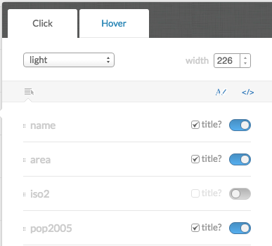
Clicking on the </> will also show the source code for the Infowindows.
<div class="cartodb-popup v2">
  <a href="#close" class="cartodb-popup-close-button close">x</a>
  <div class="cartodb-popup-content-wrapper">
    <div class="cartodb-popup-content">
      <h4>country</h4>
      <p>{{name}}</p>
      <h4>population</h4>
      <p>{{pop_norm}}</p>
      <h4>area</h4>
      <p>{{new_area}}</p>
    </div>
  </div>
  <div class="cartodb-popup-tip-container"></div>
</div>
Title, text and images:
3.4 Share your map!
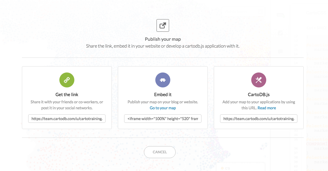
Get the link: UPDATE LINK!
https://team.cartodb.com/u/ramirocartodb/viz/0ba65c92-120b-11e6-9ab2-0e5db1731f59/public_map
Embed it:
<iframe width="100%" height="520" frameborder="0" src="https://team.cartodb.com/u/cartotraining/viz/36d25ff0-2189-11e6-b39e-0e787de82d45/embed_map" allowfullscreen webkitallowfullscreen mozallowfullscreen oallowfullscreen msallowfullscreen></iframe>
CartoDB.js
https://team.cartodb.com/u/cartotraining/api/v2/viz/36d25ff0-2189-11e6-b39e-0e787de82d45/viz.json
BONUS: JSONView, a Google Chrome extension and Pretty JSON, a Sublime Text plugin to visualize json files are good resources.
CartoDB organization features
- Your organization options
- Create/manage users of the organization
- Create groups
- Share datasets/maps with members of the organization
CartoDB Enterprise Documentation
4. Going spatial with PostGIS
4.1 Working with projections
geometry vs. geography
-
Geometryuses a cartesian plane to measure and store features (CRS units):The basis for the PostGIS
geometrytype is a plane. The shortest path between two points on the plane is a straight line. That means calculations on geometries (areas, distances, lengths, intersections, etc) can be calculated using cartesian mathematics and straight line vectors. -
Geographyuses a sphere to measure and store features (Meters):The basis for the PostGIS
geographytype is a sphere. The shortest path between two points on the sphere is a great circle arc. That means that calculations on geographies (areas, distances, lengths, intersections, etc) must be calculated on the sphere, using more complicated mathematics. For more accurate measurements, the calculations must take the actual spheroidal shape of the world into account, and the mathematics becomes very complicated indeed.
More about the geography type can be found here and here.
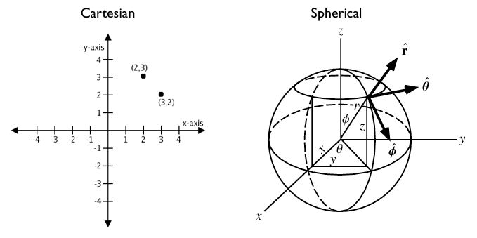
Source: Boundless Postgis intro
the_geom vs. the_geom_webmercator
the_geomEPSG:4326. Unprojected coordinates in decimal degrees (Lon/Lat). WGS84 Spheroid.the_geom_webmercatorEPSG:3857. UTM projected coordinates in meters. This is a conventional Coordinate Reference System, widely accepted as a ‘de facto’ standard in webmapping.
In CartoDB, the_geom_webmercator column is the one we see represented in the map. Know more about projections:
4.2 Changing map projections
Accessing the list of default projections available in CartoDB:
SELECT
  *
FROM
  spatial_ref_sys
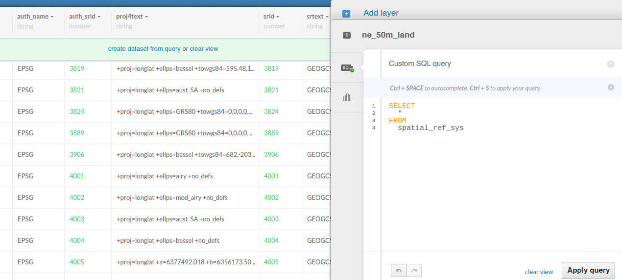
Accessing the hidden the_geom_webmercator field:
SELECT
  the_geom_webmercator
FROM
  ne_50m_land
Adding World Robinson projection (ESPG:54030):
INSERT INTO spatial_ref_sys
  (srid, auth_name, auth_srid, proj4text, srtext) values (54030, 'EPSG', 54030,
'+proj=robin +datum=WGS84','PROJCS["World_Robinson",
    GEOGCS["GCS_WGS_1984",
        DATUM["WGS_1984",
            SPHEROID["WGS_1984",6378137,298.257223563]],
        PRIMEM["Greenwich",0],
        UNIT["Degree",0.017453292519943295]],
    PROJECTION["Robinson"],
    PARAMETER["False_Easting",0],
    PARAMETER["False_Northing",0],
    PARAMETER["Central_Meridian",0],
    UNIT["Meter",1],
    AUTHORITY["EPSG","54030"]]');
ST_Transform()
SELECT
  cartodb_id, ST_Transform(the_geom, 54030) AS the_geom_webmercator
FROM
  ne_50m_land
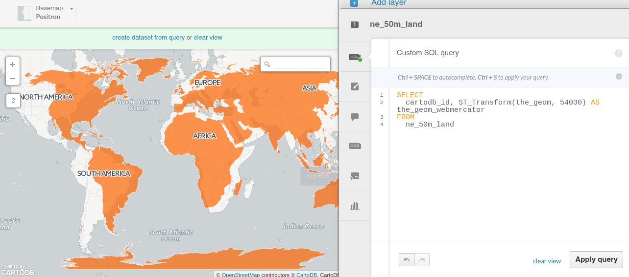
About ST_Transform.
4.3 Geoprocessing
Create a buffer from points:
SELECT
  cartodb_id,
  name,
  ST_Transform(
    ST_Buffer(the_geom::geography, 50000)::geometry
    ,3857
  ) AS the_geom_webmercator
FROM
  populated_places
WHERE
  name ilike 'madrid'
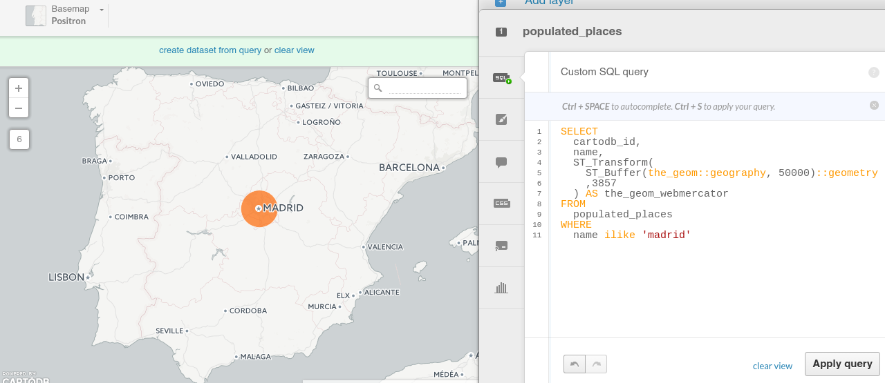
About ST_Buffer.
Note: try to compute a Buffer on a place with high latitude and check the difference between using directly the_geomwebmecator and the_geom::geography
—
Get the difference between two geometries:
SELECT
  a.cartodb_id,
    ST_Difference(
        a.the_geom_webmercator,
        b.the_geom_webmercator
  ) AS the_geom_webmercator
FROM
  ne_50m_land a,
  ne_adm0_europe b
WHERE
  b.adm0_a3 like 'ESP'
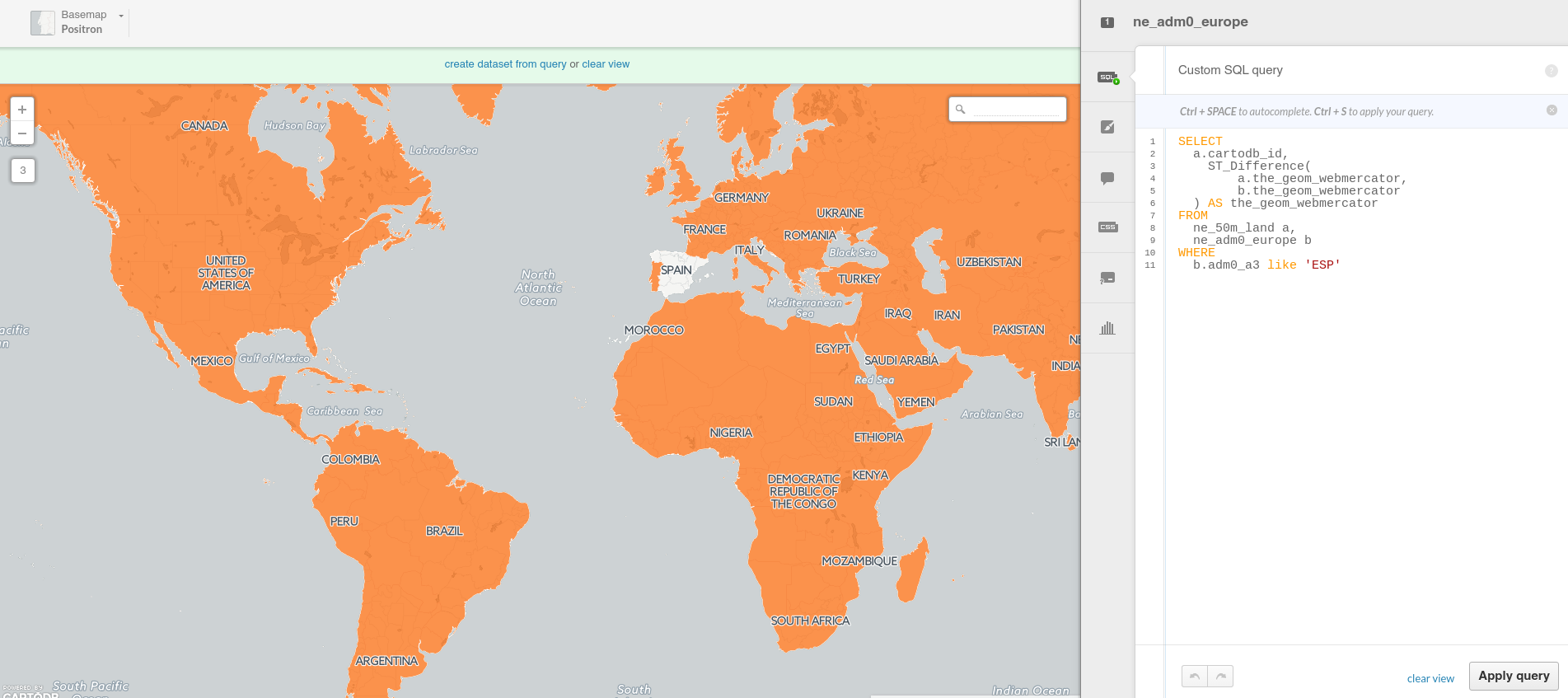
About ST_Difference.
Get the number of points inside a polygon
Using GROUP BY:
SELECT
  e.cartodb_id,
  e.admin,
  e.the_geom_webmercator,
  count(*) AS pp_count,
  sum(p.pop_max) as sum_pop
FROM
  ne_adm0_europe e
JOIN
  ne_10m_populated_places_simple p
ON
  ST_Intersects(p.the_geom, e.the_geom)
GROUP BY
  e.cartodb_id
Using LATERAL:
SELECT
  a.cartodb_id,
  a.admin AS name,
  a.the_geom_webmercator,
  counts.number_cities,
  to_char(counts.sum_pop,'999,999,999') as sum_pop --decimal separator
FROM
  ne_adm0_europe a
CROSS JOIN LATERAL
  (
    SELECT
      count(*) as number_cities,
      sum(pop_max) as sum_pop
    FROM
      ne_10m_populated_places_simple b
    WHERE
      ST_Intersects(a.the_geom, b.the_geom)
  ) AS counts
About ST_Intersects and Lateral JOIN
Note: You know about the EXPLAIN ANALYZE function? use it to take a look on how both queries are pretty similar in terms of performance.
—
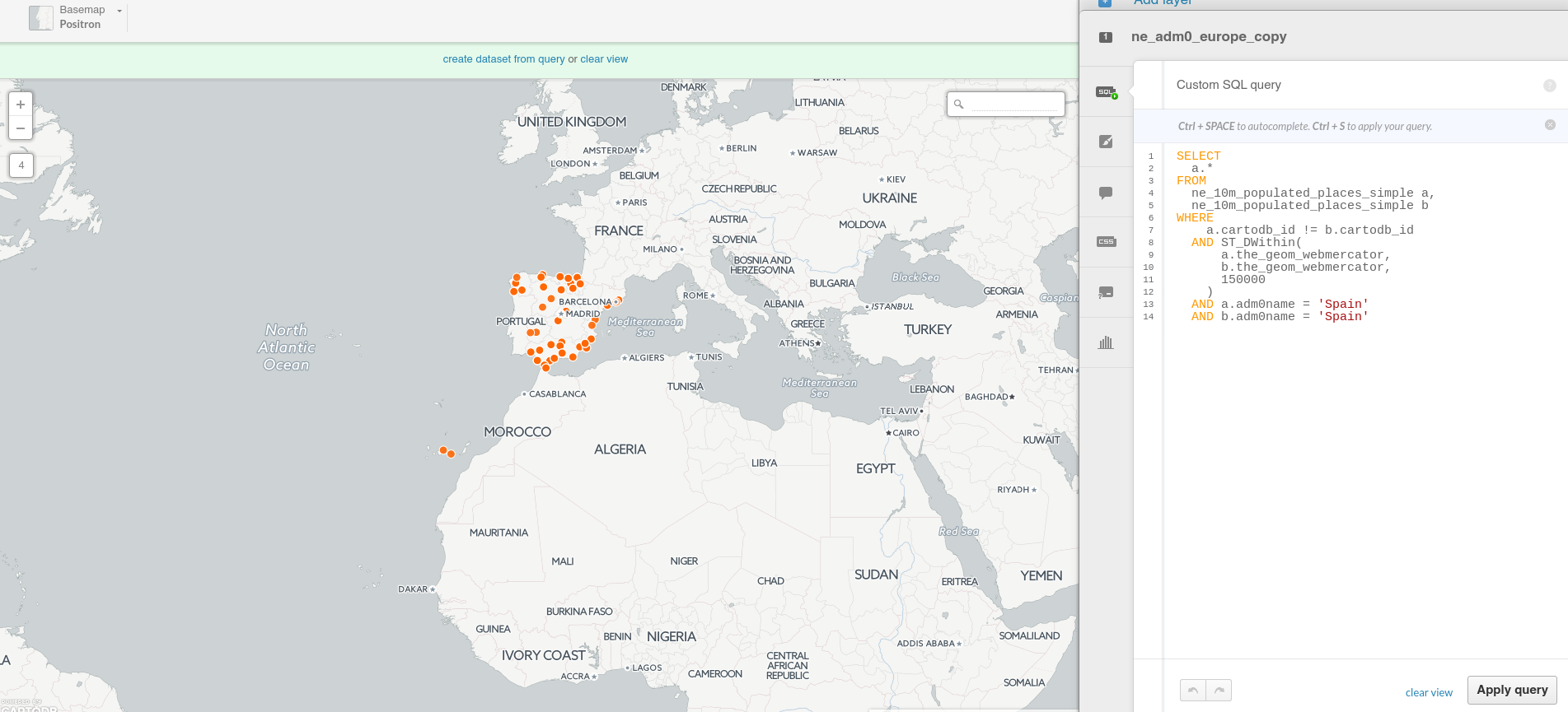
Know wether a geometry is within the given range from another geometry:
SELECT
  a.*
FROM
  ne_10m_populated_places_simple a,
  ne_10m_populated_places_simple b
WHERE
    a.cartodb_id != b.cartodb_id
  AND ST_DWithin(
      a.the_geom_webmercator,
      b.the_geom_webmercator,
      150000
    )
  AND a.adm0name = 'Spain'
  AND b.adm0name = 'Spain'
In this case, we are using the_geom_webmercator to avoid casting to geography type. Calculations made with geometry type takes the CRS units.
Keep in mind that CRS units in webmercator are not meters, and they depend directly on the latitude.
About ST_DWithin.
Create a straight line between two points:
SELECT
  ST_MakeLine(a.the_geom_webmercator,b.the_geom_webmercator) as the_geom_webmercator
FROM (SELECT * FROM populated_places
    WHERE name ILIKE 'madrid') as a,
    (SELECT * FROM populated_places
    WHERE name ILIKE 'barcelona'AND adm0name ILIKE 'spain') as b
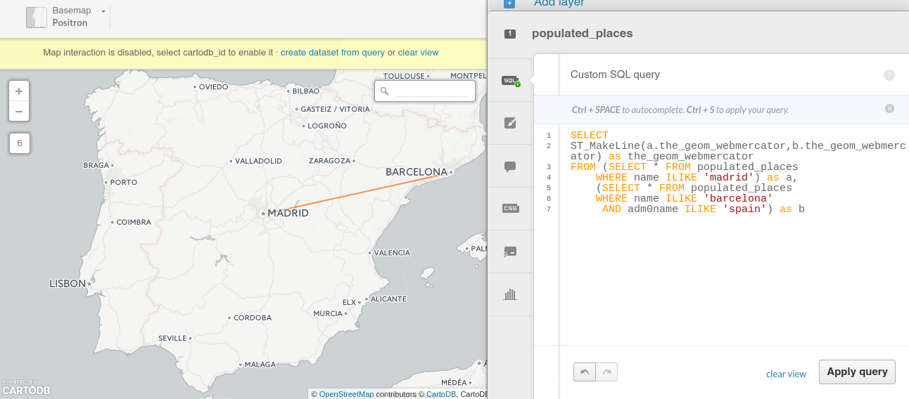
About ST_MakeLine.
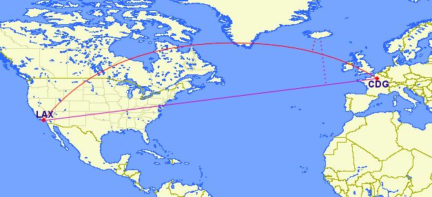
Create great circles between two points:
SELECT
  ST_Transform(
  ST_Segmentize(
      ST_Makeline(
        a.the_geom,
        b.the_geom
      )::geography,
      100000
  )::geometry,
  3857
  ) as the_geom_webmercator
FROM
  (SELECT * FROM populated_places
  WHERE name ILIKE 'madrid') as a,
  (SELECT * FROM populated_places
  WHERE name ILIKE 'new york') as b
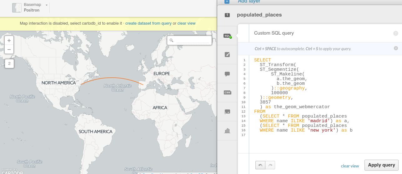
About Great Circles.
Generating Grids with CDB functions
Rectangular grid
SELECT
  row_number() over () as cartodb_id,
  CDB_RectangleGrid(
    ST_Buffer(the_geom_webmercator,125000),
  250000,
  250000
  ) AS the_geom_webmercator
FROM
  ne_adm0_europe
WHERE
  adm0_a3 IN ('ITA','GBR')
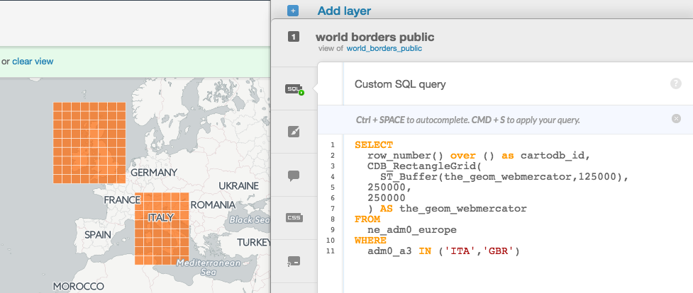
About CDB_RectangleGrid
Adaptative Hexagonal grid
WITH grid AS
(SELECT
  row_number() over () as cartodb_id,
  CDB_HexagonGrid(
    ST_Buffer(the_geom_webmercator, 100000),
    100000
  ) AS the_geom_webmercator
FROM
  ne_adm0_europe
WHERE
  adm0_a3 IN ('ESP','ITA'))

SELECT
  grid.the_geom_webmercator,
  grid.cartodb_id
FROM
  grid, ne_adm0_europe a
WHERE
    ST_intersects(grid.the_geom_webmercator, a.the_geom_webmercator)
  AND a.adm0_a3 IN ('ESP','ITA')
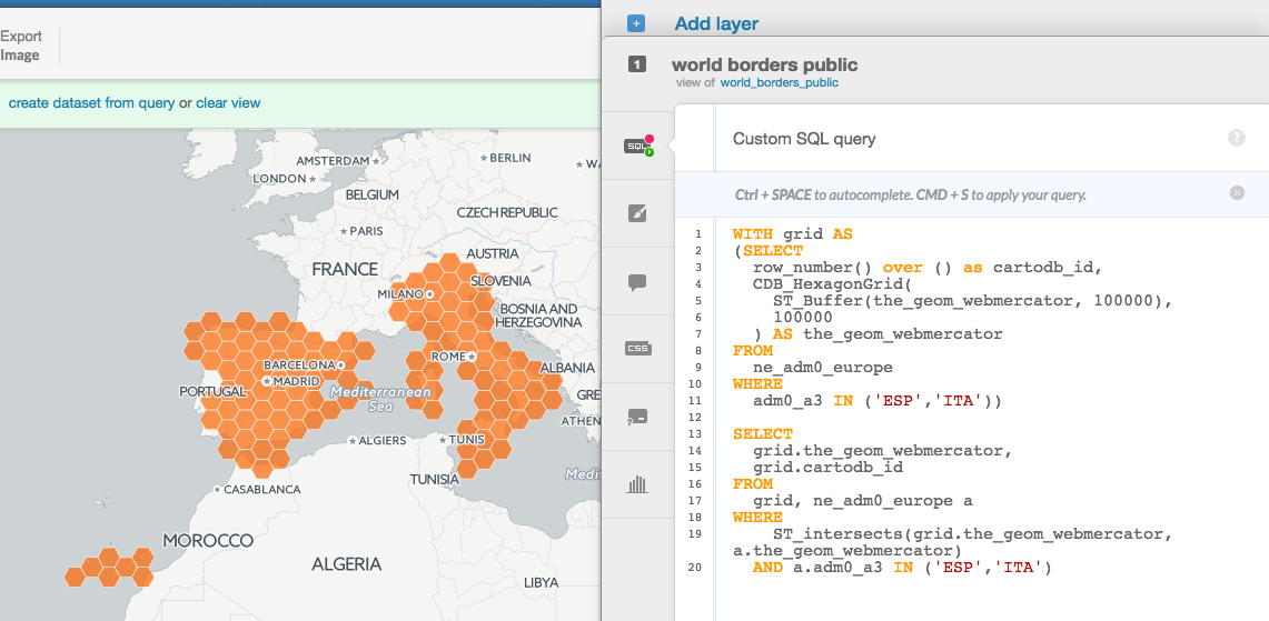
About CDB_HexagonGrid
5. Webmapping apps with CartoDB.js
5.1 CartoDB.js
CartoDB.js is the JavaScript library that allows to create webmapping apps using CartoDB services quickly and efficiently. It’s built upon the following components:
- jQuery
- Underscore.js
- Backbone.js
- It can use either Google Maps API or Leaflet
Know more about CartoDB.js here and here.
5.2 Create Visualizations and Layers
createVis()
The most basic way to display your map from CartoDB.js involves a call to:
cartodb.createVis(div_id, viz_json_url)
Couched between the <script> ... </script> tags, createVis puts a map and CartoDB data layers into the DOM element you specify. In the snippet below we assume that <div id='map'></div> placed earlier in an HTML file.
window.onload = function() {
  var vizjson = 'link from share panel';
  cartodb.createVis('map', vizjson);
}
And that’s it! All you need is that snippet of code, a script block that sources CartoDB.js, and inclusion of the CartoDB.js CSS file. It’s really one of the easiest ways to create a custom map on your webpage. createVis also accepts options that you specifiy outside of the CartoDB Editor. They take the form of a JS object, and can be passed as a third optional argument.
var options = {
  center: [40.4000, -3.6833], // Madrid
  zoom: 7,
  scrollwheel: true
};

cartodb.createVis('map', vizjson, options);
createLayer()
If you want to exercise more control over the layers and base map, createLayer may be the best option for you. You specifiy the base map yourself and load the layer from one or multiple viz.json files. Unlike createVis, createLayer needs a map object, such as one created by Google Maps or Leaflet. This difference allows for more control of the basemap for the JavaScript/HTML you’re writing.
A basic Leaflet map without your data can be created as follows:
window.onload = function() {
  // Choose center and zoom level
  var options = {
    center: [41.8369, -87.6847], // Chicago
    zoom: 7
  }

  // Instantiate map on specified DOM element
  var map = new L.Map(dom_id, options);

  // Add a basemap to the map object just created
  L.tileLayer('http://tile.stamen.com/toner/{z}/{x}/{y}.png', {
    attribution: 'Stamen'
  }).addTo(map);
}
The map we just created doesn’t have any CartoDB data layers yet. If you’re just adding a single layer, you can put your data on top of the basemap from above. If you want to add more, you just repeat the process. We’ll be doing much more with this later. This is the basic snippet to put your data on top of the map you just created. Drop this in below the L.tileLayer section.
var vizjson = 'link from share panel';
cartodb.createLayer(map, vizjson).addTo(map);
5.3 UI Functions
Tooltips
A tooltip is an infowindow that appears when you hover your mouse over a map feature with vis.addOverlay(options). A tooltip appears where the mouse cursor is located on the map.
To add a tooltip to a map you need to do two steps:
First, define tooltip variable:
  var tooltip = layer.leafletMap.viz.addOverlay({
            type: 'tooltip',
            layer: layer,
            template: '<div class="cartodb-tooltip-content-wrapper"><p>{{name}}</p></div>',
            width: 200,
            position: 'bottom|right',
            fields: [{ name: 'name' }]
  });
Second, add tooltip to the map:
$('body').append(tooltip.render().el);
Infowindows
Infowindows provide additional interactivity for your published map, controlled by layer events. It enables interaction and overrides the layer interactivity. A pop-up information window appears when a viewer clicks on a map feature.
In order to add the CartoDB.js infowindow you need to add this line within your code:
cdb.vis.Vis.addInfowindow(map, layer, ['fields']);
However, you can create custom infowindows with different tools (Moustache.js, HTML or underscore.js). Whatever choice you make, you would need to create a template first and then add the infowindow with the template. Here we will see how to do it using Moustache.js.
Mustache.js is a logic-less logic-template. That means that only tags you create templates that are replaced with a value or series of values, it works by expanding tags in a template using values provided in a hash or object.
Example: Custom infowindow template to display cartodb_id:
  <script type="infowindow/html" id="infowindow_template">
    <div class="cartodb-popup v2">
  <a href="#close" class="cartodb-popup-close-button close">x</a>
  <div class="cartodb-popup-content-wrapper">
    <div class="cartodb-popup-content">
      <h4>ID</h4>
      <p>{{cartodb_id}}</p>
    </div>
  </div>
  <div class="cartodb-popup-tip-container"></div>
</div>
</script>
Then you can apply the custom infowindow template to the map with:
cdb.vis.Vis.addInfowindow(
          map, layer, [columnName],
          {
             infowindowTemplate: $('#infowindow_template').html()
          });
Legends
In order to add legends with CartoDB.js you would need to define the elemenets and colors of the legend with HTML, then you could use the legend classes of CartoDB.js to create the legends.
There are two kind of legend classes:
First, cartodb-legend choropleth, applied in Choropleth maps:
<div class='cartodb-legend choropleth'>
    <div class="legend-title">Population</div>
      <ul>
      	<li class="min">
      		1256
      	</li>
      	<li class="max">
      		8300
      	</li>
      	<li class="graph count_441">
      	<div class="colors">
      	<div class="quartile" style="background-color:#FFFFB2"></div>
      	<div class="quartile" style="background-color:#FED976"></div>
      	<div class="quartile" style="background-color:#FEB24C"></div>
      	<div class="quartile" style="background-color:#FD8D3C"></div>
      	<div class="quartile" style="background-color:#FC4E2A"></div>
      	<div class="quartile" style="background-color:#E31A1C"></div>
      	<div class="quartile" style="background-color:#B10026"></div>
      	</div>
      	</li>
      </ul>
  </div>
Second, cartodb-legend category, applied in simple or category maps:
    <div class='cartodb-legend category'>
      <div class="legend-title" style="color:#284a59">Countries</div>
        <ul>
          <li><div class="bullet" style="background-color:#fbb4ae"></div>Spain</li>
          <li><div class="bullet" style="background-color:#ccebc5"></div>Portugal</li>
          <li><div class="bullet" style="background-color:#b3cde3"></div>France</li>
        </ul>
      </div>
5.4 Examples
Some more advanced examples
- Playing with Torque time
- Aggregating content from clustered features with SQL
- Creating a simple layer selector