CartoDB Workshops : CartoDB Intro Workshop for Madlan

This introductory workshop was given by Ramiro Aznar on June 23, 2016 at . As taught, it was 2h hours long.

Trainer: Ramiro Aznar · ramiroaznar@cartodb.com · @ramiroaznar
June 23th 2016
CartoDB Introductory Workshop for Madlan

http://bit.ly/madlan

Map Academy, tutorials and other online resources

Further questions and troubleshooting

Email to support@cartodb.com.
Some questions could be already anwered at GIS Stack Exchange cartodb tag.

Importing datasets
Getting your data ready
Making a map

1. Importing datasets

1.1 Supported Geospatial Data Files

CartoDB supports the following geospatial data formats to upload vector data*:

Shapefile
KML
KMZ
GeoJSON*
CSV
Spreadsheets
GPX
OSM

Importing different geometry types in the same layer or in a FeatureCollection element (GeoJSON) is not supported. More detailed information here.

[*] More detailed information about GeoJSON format here, here and here.

1.2 Common importing errors

Dataset too large:
- File size limit: 150 Mb (free).
- Import row limit: 500,000 rows (free).
- Solution: split your dataset into smaller ones, import them into CartoDB and merge them.
Malformed CSV:
- Solution: check termination lines, header…
Encoding:
- Solution: Save with Encoding > UTF-8 with BOM in Sublime Text, any other decent text editor or iconv.
Shapefile missing files:
- Missing any of the following files within the compressed file will produce an importing error:
  - .shp: contains the geometry. REQUIRED.
  - .shx: contains the shape index. REQUIRED.
  - .prj: contains the projection. REQUIRED.
  - .dbf: contains the attributes. REQUIRED.
- Other auxiliary files such as .sbn, .sbx or .shp.xml are not REQUIRED.
- Solution: make sure to add all required files.
Duplicated id fields:
- Solution: check your dataset, remove or rename fields containing the id keyword.
Format not supported:
- URLs -that are not points to a file- are not supported by CartoDB.
- Solution: check for missing url parameters or download the file into your local machine, import it into CartoDB.
Non supported SRID:
- Solution: try to reproject your resources locally to a well known projection like EPSG:4326,EPSG:3857,EPSG:25830 and so on.

Other importing errors and their codes can be found here.

2. Getting your data ready

2.1 Geocoding

If you have a column with longitude coordinates and another with latitude coordinates, CartoDB will automatically detect and covert values into the_geom. If this is not the case, CartoDB can help you by turning the named places into best guess of latitude-longitude coordinates:

By Lon/Lat Columns.
By City Names.
By Admin. Regions.
By Postal Codes.
By IP Addresses.
By Street Addresses.

Know more about geocoding in CartoDB here.

2.2 Datasets

These are the datasets we are going to use on our workshop. You’ll find them all on our Data Library:

Populated Places [ne_10m_populated_places_simple]: City and town points.
World Borders [world_borders]: World countries borders.

2.3 Simple SQL operations

Selecting all columns:

SELECT
  *
FROM
  ne_10m_populated_places_simple;

Selecting some columns:

SELECT
  cartodb_id,
  name as city,
  adm1name as region,
  adm0name as country,
  pop_max,
  pop_min
FROM
  ne_10m_populated_places_simple

Selecting distinct values:

SELECT DISTINCT
  adm0name as country
FROM
  ne_10m_populated_places_simple

2.4 Filtering

filtering

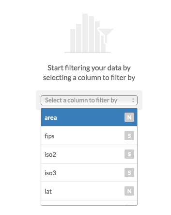
Filtering numeric fields:

SELECT
  *
FROM
  ne_10m_populated_places_simple
WHERE
  pop_max > 5000000;

Filtering character fields:

SELECT
  *
FROM
  ne_10m_populated_places_simple
WHERE
  adm0name ilike 'spain'

Filtering a range:

SELECT
  *
FROM
  ne_10m_populated_places_simple
WHERE
  name in ('Madrid', 'Barcelona')
AND
  adm0name ilike 'spain'

Combining character and numeric filters:

SELECT
  *
FROM
  ne_10m_populated_places_simple
WHERE
  name in ('Madrid', 'Barcelona')
AND
  adm0name ilike 'spain'
AND
  pop_max > 5000000

2.5 Others:

Selecting aggregated values:

count

SELECT
  count(*) as total_rows
FROM
  ne_10m_populated_places_simple

sum

SELECT
  sum(pop_max) as total_pop_spain
FROM
  ne_10m_populated_places_simple
WHERE
  adm0name ilike 'spain'

avg

SELECT
  avg(pop_max) as avg_pop_spain
FROM
  ne_10m_populated_places_simple
WHERE
  adm0name ilike 'spain'

Ordering results:

SELECT
  cartodb_id,
  name as city,
  adm1name as region,
  adm0name as country,
  pop_max
FROM
  ne_10m_populated_places_simple
WHERE
  adm0name ilike 'spain'
ORDER BY
  pop_max DESC

Limiting results:

SELECT
  cartodb_id,
  name as city,
  adm1name as region,
  adm0name as country,
  pop_max
FROM
  ne_10m_populated_places_simple
WHERE
  adm0name ilike 'spain'
ORDER BY
  pop_max DESC
LIMIT 10

3. Making our first map

3.1 Wizard

Analyzing your dataset… In some cases, when you connect a dataset and click on the MAP VIEW for the first time, the Analyzing dataset dialog appears. This analytical tool analyzes the data in each column, predicts how to visualize this data, and offers you snapshots of the visualized maps. You can select one of the possible map styles, or ignore the analyzing dataset suggestions.

Simple Map
Cluster Map
Category Map
Bubble Map
Torque Map
Heatmap Map
Torque Cat Map
Intensity Map
Density Map
Choropleth Map:

Know more about chosing the right map to make here.

3.2 Styles

The last link in the website referenced above is a great discussion about the different maps CartoDB allows to create.

Simple Map:

/** simple visualization */

#layer{
  polygon-fill: #FF6600;
  polygon-opacity: 0.7;
  line-color: #FFF;
  line-width: 0.5;
  line-opacity: 1;
}

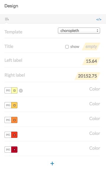
Choropleth Map:

Before making a choropleth map, we need to normalize our target column. For that, we need to divide the population by the area.

SELECT
  wb.*,
  pop2005/(ST_Area(the_geom::geography)/1000000) AS pop_norm
FROM
  world_borders wb

Click on ‘create new dataset from query’.

Rename the new dataset to world_borders_norm

choropleth

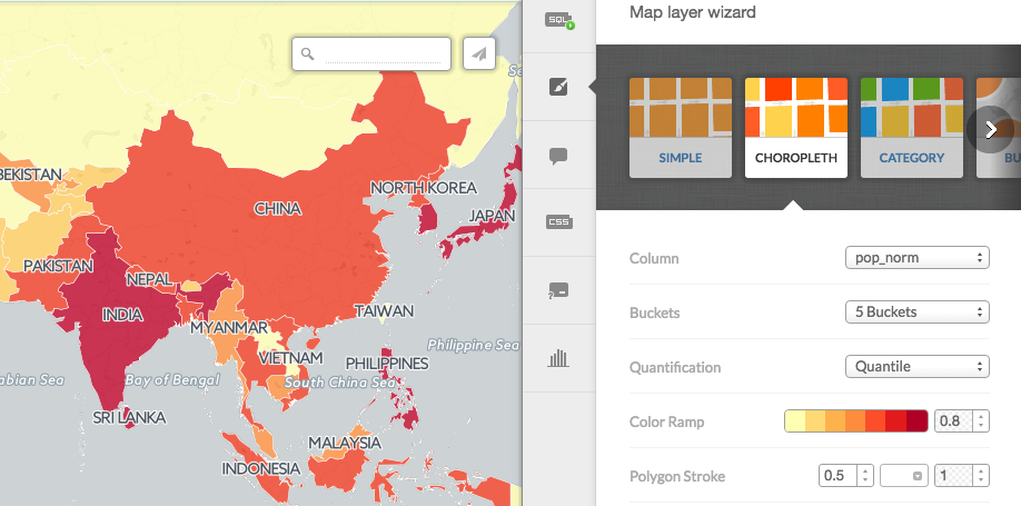
/** choropleth visualization */

#layer{
  polygon-fill: #FFFFB2;
  polygon-opacity: 0.8;
  line-color: #FFF;
  line-width: 0.5;
  line-opacity: 1;
}
#layer [ pop_norm <= 247992435.530086] {
   polygon-fill: #B10026;
}
#layer [ pop_norm <= 4086677.23673585] {
   polygon-fill: #E31A1C;
}
#layer [ pop_norm <= 1538732.3943662] {
   polygon-fill: #FC4E2A;
}
#layer [ pop_norm <= 923491.374542489] {
   polygon-fill: #FD8D3C;
}
#layer [ pop_norm <= 616975.331234902] {
   polygon-fill: #FEB24C;
}
#layer [ pop_norm <= 326396.192958792] {
   polygon-fill: #FED976;
}
#layer [ pop_norm <= 95044.5589361554] {
   polygon-fill: #FFFFB2;
}

Proportional symbols map

Take a look on this excellent blog post by Mamata Akella regarding how to produce proportional symbols maps. The easiest ones being buble maps since it’s directly supported by CartoDB wizards. The other type, the graduated symbols where you compute the radius of the symbol to be used later on the CartoCSS* section needs a bit of SQL computation but nothing hard.

WITH aux AS(
  SELECT
    max(pop2005) AS max_pop
  FROM
    world_borders
  )
SELECT
  cartodb_id,
  pop2005,
  ST_Centroid(the_geom_webmercator) AS the_geom_webmercator,
  5+30*sqrt(pop2005)/sqrt(aux.max_pop) AS size
FROM
  world_borders,
  aux

#layer{
  marker-fill-opacity: 0.8;
  marker-line-color: #FFF;
  marker-line-width: 1;
  marker-line-opacity: 1;
  marker-width: [size];
  marker-fill: #FF9900;
  marker-allow-overlap: true;
}

[*] Know more about CartoCSS with our documentation and try our cartoColors!

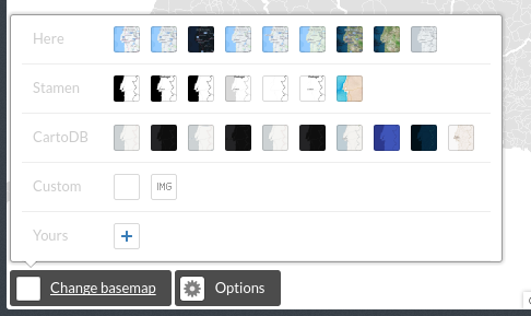
3.3 Other elements

Basemaps:

basemap

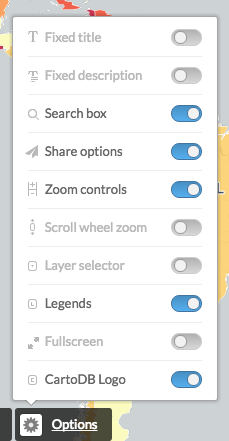
Options:

options

Legend:

legend

By clicking on the </> icon, you would see and edit the source HTML code.

<div class='cartodb-legend choropleth'>
<div class="legend-title">Total Population</div>
<ul>
	<li class="min">
		95044.56
	</li>
	<li class="max">
		247992435.53
	</li>
	<li class="graph count_441">
	<div class="colors">
	<div class="quartile" style="background-color:#FFFFB2"></div>
	<div class="quartile" style="background-color:#FED976"></div>
	<div class="quartile" style="background-color:#FEB24C"></div>
	<div class="quartile" style="background-color:#FD8D3C"></div>
	<div class="quartile" style="background-color:#FC4E2A"></div>
	<div class="quartile" style="background-color:#E31A1C"></div>
	<div class="quartile" style="background-color:#B10026"></div>
	</div>
	</li>
</ul>
</div>

Labels:

intensity

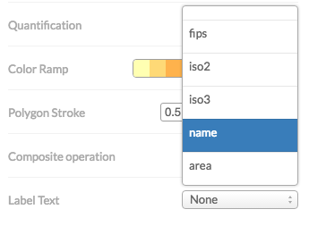
Selecting a field in the wizard will produce the following CartoCSS code to render the labels.

#world_borders::labels {
  text-name: [name];
  text-face-name: 'DejaVu Sans Book';
  text-size: 10;
  text-label-position-tolerance: 10;
  text-fill: #000;
  text-halo-fill: #FFF;
  text-halo-radius: 1;
  text-dy: -10;
  text-allow-overlap: true;
  text-placement: point;
  text-placement-type: simple;
}

This also shows an important concept for CartoCSS. you can specify more than one rendering pass for your features. This means that using the #layername::passname notation you can render more than one symbol on your features.

infowindows

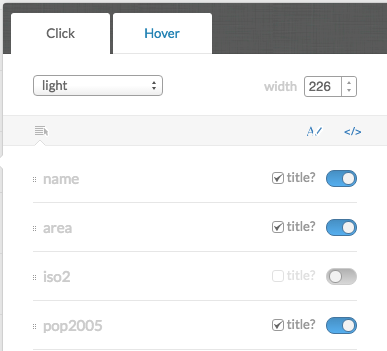
Clicking on the </> will also show the source code for the Infowindows.

<div class="cartodb-popup v2">
  <a href="#close" class="cartodb-popup-close-button close">x</a>
  <div class="cartodb-popup-content-wrapper">
    <div class="cartodb-popup-content">
      <h4>country</h4>
      <p>{{name}}</p>
      <h4>population</h4>
      <p>{{pop_norm}}</p>
      <h4>area</h4>
      <p>{{new_area}}</p>
    </div>
  </div>
  <div class="cartodb-popup-tip-container"></div>
</div>

Title, text and images:

elements

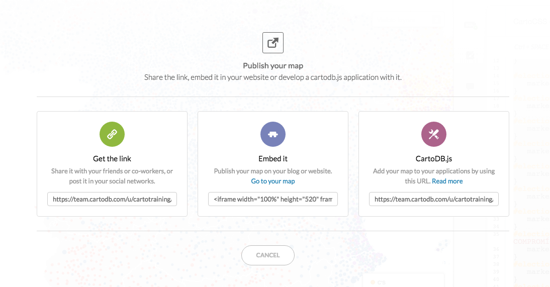
Get the link:

https://team.cartodb.com/u/cartotraining/viz/36d25ff0-2189-11e6-b39e-0e787de82d45/public_map

Embed it:

<iframe width="100%" height="520" frameborder="0" src="https://team.cartodb.com/u/cartotraining/viz/36d25ff0-2189-11e6-b39e-0e787de82d45/embed_map" allowfullscreen webkitallowfullscreen mozallowfullscreen oallowfullscreen msallowfullscreen></iframe>

CartoDB Workshops Materials for Teaching Maps

CartoDB Intro Workshop for Madlan

http://bit.ly/madlan

Map Academy, tutorials and other online resources

Further questions and troubleshooting

Contents

1. Importing datasets

1.1 Supported Geospatial Data Files

1.2 Common importing errors

2. Getting your data ready

2.1 Geocoding

2.2 Datasets

2.3 Simple SQL operations

Selecting all columns:

Selecting some columns:

Selecting distinct values:

2.4 Filtering

Filtering numeric fields:

Filtering character fields:

Filtering a range:

Combining character and numeric filters:

2.5 Others:

Selecting aggregated values:

Ordering results:

Limiting results:

3. Making our first map

3.1 Wizard

3.2 Styles

Simple Map:

Choropleth Map:

Proportional symbols map

3.3 Other elements

Basemaps:

Options:

Legend:

Labels:

Infowindows and tooltip:

Title, text and images:

Get the link:

Embed it:

CartoDB Workshops Materials for Teaching Maps

CartoDB Intro Workshop for Madlan

http://bit.ly/madlan

Map Academy, tutorials and other online resources

Further questions and troubleshooting

Contents

1. Importing datasets

1.1 Supported Geospatial Data Files

1.2 Common importing errors

2. Getting your data ready

2.1 Geocoding

2.2 Datasets

2.3 Simple SQL operations

Selecting all columns:

Selecting some columns:

Selecting distinct values:

2.4 Filtering

Filtering numeric fields:

Filtering character fields:

Filtering a range:

Combining character and numeric filters:

2.5 Others:

Selecting aggregated values:

Ordering results:

Limiting results:

3. Making our first map

3.1 Wizard

3.2 Styles

Simple Map:

Choropleth Map:

Proportional symbols map

3.3 Other elements

Basemaps:

Options:

Legend:

Labels:

Infowindows and tooltip:

Title, text and images:

3.4 Share your map!

Get the link:

Embed it: